Normal models and linear combinations
Interpret normal areas and inverse tails, recover parameters, and compare transformed or independent measurements under a model.
Practise
More
Offline pages
Saved on this device only. Connect at least once every 30 days to confirm Premium. Sign-out or a change of account removes saved copies.
Find this activity in your course
On this page
You stopped at:
ContinueRevision Mode is on. Questions and activities are hidden.
The second parameter is variance
Write X∼ N(μ,σ²) for a normal model with mean μ and positive standard deviation σ. The second parameter is the variance, not the standard deviation. Thus X∼ N(100,225) has mean 100, variance 225 and standard deviation 15.
The density curve is symmetric about μ and has its peak there. Its total area is one. Moving μ shifts the whole curve; increasing σ spreads the area across a wider range and lowers the peak. A larger peak does not mean a larger total probability.
A normal model is continuous. Probability is area below its density curve over an interval; the height at one point is not a probability. Every single value has probability zero, so P(X = x) = 0 and P(X < x) = P(X ≤ x) for any exact boundary x. Symmetry gives P(X < μ) = P(X > μ) = 1/2.
An instrument’s displayed reading is a different event from an exact value. If it rounds to the nearest whole unit, a displayed 100 represents values from 99.5 to 100.5, apart from the irrelevant choice of which interval owns an exact halfway point. That interval can have positive probability even though P(X = 100) = 0.
Standardise the boundary and keep the event
Subtracting the mean centres a normal variable at zero. Dividing by its standard deviation measures distance in standard deviations:
For X∼ N(100,225), a boundary of 130 is two standard deviations above the mean. Since σ = 15 is positive, standardising preserves the inequality:
Dividing by 225 would use the variance in place of the standard deviation and place the boundary in the wrong part of the curve. The small upper-tail probability agrees with a boundary well above the mean.
At X = 122.5, the standardised boundary is 1.5, and P(X > 122.5) = P(Z > 1.5) ≈ 0.0668072. In the figure, locate the area below the solid curve and to the right of the dashed boundary. The vertical segment identifies the boundary; its height is not the answer.
Locate a right-tail probability on a normal density
The density is symmetric about zero, with a peak of approximately 0.398942 at zero. It decreases towards zero in either direction. At z = 1.5 the density is approximately 0.129518; the probability to the right is an area, not that height. The dashed segment runs from the horizontal axis to the curve at z = 1.5.
Scroll across the figure to read all labels.
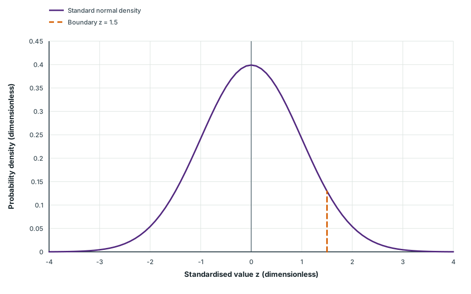
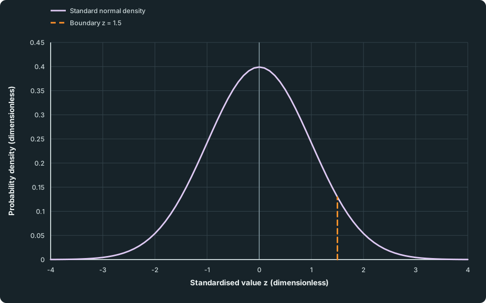
View figure data
| Series | Standardised value z (dimensionless) | Probability density (dimensionless) |
|---|---|---|
| Standard normal density | -4.0 | 0.0001338 |
| Standard normal density | -3.9 | 0.0001987 |
| Standard normal density | -3.8 | 0.0002919 |
| Standard normal density | -3.7 | 0.0004248 |
| Standard normal density | -3.6 | 0.0006119 |
| Standard normal density | -3.5 | 0.0008727 |
| Standard normal density | -3.4 | 0.0012322 |
| Standard normal density | -3.3 | 0.0017226 |
| Standard normal density | -3.2 | 0.0023841 |
| Standard normal density | -3.1 | 0.0032668 |
| Standard normal density | -3.0 | 0.0044318 |
| Standard normal density | -2.9 | 0.0059525 |
| Standard normal density | -2.8 | 0.0079155 |
| Standard normal density | -2.7 | 0.0104209 |
| Standard normal density | -2.6 | 0.0135830 |
| Standard normal density | -2.5 | 0.0175283 |
| Standard normal density | -2.4 | 0.0223945 |
| Standard normal density | -2.3 | 0.0283270 |
| Standard normal density | -2.2 | 0.0354746 |
| Standard normal density | -2.1 | 0.0439836 |
| Standard normal density | -2.0 | 0.0539910 |
| Standard normal density | -1.9 | 0.0656158 |
| Standard normal density | -1.8 | 0.0789502 |
| Standard normal density | -1.7 | 0.0940491 |
| Standard normal density | -1.6 | 0.1109208 |
| Standard normal density | -1.5 | 0.1295176 |
| Standard normal density | -1.4 | 0.1497275 |
| Standard normal density | -1.3 | 0.1713686 |
| Standard normal density | -1.2 | 0.1941861 |
| Standard normal density | -1.1 | 0.2178522 |
| Standard normal density | -1.0 | 0.2419707 |
| Standard normal density | -0.9 | 0.2660852 |
| Standard normal density | -0.8 | 0.2896916 |
| Standard normal density | -0.7 | 0.3122539 |
| Standard normal density | -0.6 | 0.3332246 |
| Standard normal density | -0.5 | 0.3520653 |
| Standard normal density | -0.4 | 0.3682701 |
| Standard normal density | -0.3 | 0.3813878 |
| Standard normal density | -0.2 | 0.3910427 |
| Standard normal density | -0.1 | 0.3969525 |
| Standard normal density | 0.0 | 0.3989423 |
| Standard normal density | 0.1 | 0.3969525 |
| Standard normal density | 0.2 | 0.3910427 |
| Standard normal density | 0.3 | 0.3813878 |
| Standard normal density | 0.4 | 0.3682701 |
| Standard normal density | 0.5 | 0.3520653 |
| Standard normal density | 0.6 | 0.3332246 |
| Standard normal density | 0.7 | 0.3122539 |
| Standard normal density | 0.8 | 0.2896916 |
| Standard normal density | 0.9 | 0.2660852 |
| Standard normal density | 1.0 | 0.2419707 |
| Standard normal density | 1.1 | 0.2178522 |
| Standard normal density | 1.2 | 0.1941861 |
| Standard normal density | 1.3 | 0.1713686 |
| Standard normal density | 1.4 | 0.1497275 |
| Standard normal density | 1.5 | 0.1295176 |
| Standard normal density | 1.6 | 0.1109208 |
| Standard normal density | 1.7 | 0.0940491 |
| Standard normal density | 1.8 | 0.0789502 |
| Standard normal density | 1.9 | 0.0656158 |
| Standard normal density | 2.0 | 0.0539910 |
| Standard normal density | 2.1 | 0.0439836 |
| Standard normal density | 2.2 | 0.0354746 |
| Standard normal density | 2.3 | 0.0283270 |
| Standard normal density | 2.4 | 0.0223945 |
| Standard normal density | 2.5 | 0.0175283 |
| Standard normal density | 2.6 | 0.0135830 |
| Standard normal density | 2.7 | 0.0104209 |
| Standard normal density | 2.8 | 0.0079155 |
| Standard normal density | 2.9 | 0.0059525 |
| Standard normal density | 3.0 | 0.0044318 |
| Standard normal density | 3.1 | 0.0032668 |
| Standard normal density | 3.2 | 0.0023841 |
| Standard normal density | 3.3 | 0.0017226 |
| Standard normal density | 3.4 | 0.0012322 |
| Standard normal density | 3.5 | 0.0008727 |
| Standard normal density | 3.6 | 0.0006119 |
| Standard normal density | 3.7 | 0.0004248 |
| Standard normal density | 3.8 | 0.0002919 |
| Standard normal density | 3.9 | 0.0001987 |
| Standard normal density | 4.0 | 0.0001338 |
| Boundary z = 1.5 | 1.5 | 0.0000000 |
| Boundary z = 1.5 | 1.5 | 0.1295176 |
For a two-boundary event, standardise both ends before subtracting lower-tail probabilities. For example, 85 < X < 130 becomes -1 < Z < 2, so
A calculator can instead evaluate the original interval using lower bound 85, upper bound 130, mean 100 and standard deviation 15. Check the command’s parameter order and whether it expects σ or σ². Use its infinity facility for an unbounded tail, where available, rather than treating an arbitrary finite cutoff as the event’s exact boundary. Both methods should describe the same area.
Check your understanding 1 Distinguish a point from a reported interval
For X∼ N(100,225), find P(85 < X < 130) and P(X ≥ 130) to three significant figures. Then find the probability that an instrument rounding X to the nearest whole unit displays 100. Explain why that last probability differs from P(X = 100).
Show answer
The interval probability is P(Z < 2)-P(Z < -1) ≈ 0.819. The upper tail is P(Z ≥ 2) ≈ 0.0228. Including the exact endpoint changes neither probability because a single value has zero probability under this continuous model.
A displayed 100 means 99.5 ≤ X < 100.5, so use standardised bounds -0.5/15 and 0.5/15. The probability is approximately 0.0265912, or 0.0266 to three significant figures. By contrast, P(X = 100) = 0. Rounding collects an interval of underlying values; it does not turn the continuous model into a point mass at 100.
Condition on the event that was observed
A conditional probability restricts the experiments being considered. For X∼ N(100,225), let A be the event X > 130 and B the event X > 100. Every result in A is also in B, so
The numerator uses the intersection, and dividing by P(B) rescales that probability within B. A and B are not independent here: knowing that X is above 130 guarantees it is above 100. Conditioning on X > 100 also restricts the original normal distribution; it does not leave an unrestricted N(100,225) model for the selected values.
Check your understanding 2 Intersect two overlapping events
For X∼ N(100,225), find P(85 < X < 130 ∣ X > 100) to three significant figures. Write the numerator’s event and the denominator before calculating. Explain why using the probability of 85 < X < 130 as the numerator would include excluded values.
Show answer
The intersection is 100 < X < 130. Its standardised event is 0 < Z < 2, with probability approximately 0.4772499. The condition X > 100 has probability 0.5, so the conditional probability is P(0 < Z < 2)/0.5 ≈ 0.9544997, or 0.954 to three significant figures. Using 85 < X < 130 would also count values below 100, which do not satisfy the condition. Including or excluding a single endpoint changes none of these probabilities under the continuous model.
Inverse probabilities recover a boundary
An inverse normal command works in the opposite direction: an area gives a boundary. Check which tail its input represents. For a standard normal lower-tail inverse, input 0.975 gives z ≈ 1.95996398, while input 0.025 gives z ≈ -1.95996398. Symmetry puts them on opposite sides of zero.
Thus an upper-tail probability of 0.025 uses lower-tail input 0.975, not 0.025. For a general normal variable, convert the resulting standardised boundary back with
For example, the central 95% interval leaves 2.5% in each tail, so its boundaries are approximately μ-1.95996σ and μ + 1.95996σ. The upper boundary is the 97.5th percentile, not the 95th percentile. Equal tails matter here; “an interval containing 95%” alone does not specify a unique interval.
If the mean is 100 and P(X < 124) = 0.975, then
where z_(0.975) ≈ 1.95996398 is the standard normal boundary with lower-tail probability 0.975. Hence σ = 24/z_(0.975) ≈ 12.2451 and σ² ≈ 149.943. Use the unrounded inverse result when squaring: a standard deviation and a variance are different requested answers.
A probability also constrains the signs. With mean 100 and positive σ, the boundary 124 lies above the mean, so its lower-tail probability must exceed one half. A claim that P(X < 124) = 0.2 would contradict this normal model; replacing a negative computed σ by its absolute value would not repair the probability statement.
Check your understanding 3 Recover both location and spread
A normal variable has P(X < 88) = 0.1 and P(X > 118) = 0.05. Find its mean and variance, each to three decimal places. Write the two standardised boundary equations before solving, and check the signs and ordering of the boundaries.
Show answer
The standard normal lower-tail boundaries are z_(0.1) ≈ -1.28155157 and z_(0.95) ≈ 1.64485363. The second uses 0.95 because the given upper tail is 0.05.
The equations are 88 = μ + z_(0.1)σ and 118 = μ + z_(0.95)σ. Subtracting gives 30 = (z_(0.95)-z_(0.1))σ, hence σ ≈ 10.25148536 and μ ≈ 101.13780712. The requested mean is 101.138 and the variance is 105.093 to three decimal places.
The recovered mean lies between 88 and 118, and σ is positive. Substituting the unrounded parameters gives the original lower-tail probabilities 0.1 and 0.95. Using 0.05 directly for the second lower-tail inverse would put both standardised boundaries below zero and solve a different problem.
Transform location and spread differently
For constants a and b,
Adding b shifts all values by the same amount, so it changes the mean without changing spread. Multiplying deviations by a multiplies their squares by a². The standard deviation therefore scales by |a|, even if a is negative.
For normal X and a non-zero a, the transformed variable is also normal, with these transformed parameters. If a = 0, the result is the constant b with variance zero; it is not a normal variable with a positive standard deviation, and cannot be standardised by dividing by zero.
Check your understanding 4 Variance does not transform linearly
For X∼ N(8,9), find the mean and variance of Y = 4 − 2X, and calculate P(Y > 0) to three significant figures. Then find Var(X + Y). Can you add Var(X) and Var(Y) for this last calculation?
Show answer
The mean is 4 − 16 = −12 and variance is (−2)²(9) = 36, so Y∼ N(-12,36) with standard deviation 6. Thus P(Y > 0) = P(Z > 2) ≈ 0.0228.
Alternatively, 4-2X > 0 means X < 2: division by the negative coefficient reverses the inequality. This gives P(Z < -2), the same probability by symmetry.
Since Y is defined from the same X, they are dependent. Rewrite X + Y = 4-X, so Var(X + Y) = (−1)²(9) = 9. Adding 9 and 36 as though they came from independent draws would give the incorrect 45. The negative multiplier reverses value order; it does not make a negative variance.
Combine independent observations before finding a probability
For independent X and Y with finite variances,
The expectation rule does not need independence, but the displayed variance addition does need independence or another justified reason for a zero dependence contribution. If X and Y are independent normal variables, their linear combination is normal whenever its variance is positive. Without independence, their separate normal distributions alone do not settle the variance or the distribution of the combination.
For independent X∼ N(10,4) and Y∼ N(20,9), let D = 2X − Y. Its mean is 2(10) − 20 = 0 and its variance is 2²(4) + (-1)²(9) = 25. Thus D∼ N(0,25) and P(D > 5) = P(Z > 1) ≈ 0.158655. The minus sign subtracts a mean, while its squared coefficient adds a positive variance contribution.
A fresh observation also differs from a repeated use of one value. If X₁ and X₂ are independent, each with model N(10,4), then X₁ + X₂∼ N(20,8). But 2X₁∼ N(20,16). Their means agree, yet P(X₁ + X₂ > 24) ≈ 0.0786496, while P(2X₁ > 24) ≈ 0.158655.
Before adding variances, write the physical observation represented by each variable. Different letters do not themselves establish independence; measurements from a common varying source can remain related.
Check whether the model is plausible
A normal distribution extends across the whole real line. It may still model a non-negative measurement usefully when its negative tail is negligible in that setting. Plausibility also depends on the measurement process and the observed shape: a symmetric bell shape should not be assumed from a mean and variance alone.
Check your understanding 5 Does the tail fit a waiting-time model?
A waiting time T in minutes is proposed to have model N(1,4). Calculate its probability of a negative waiting time, to three significant figures. Explain whether the model is plausible for these waiting times and whether simply discarding all negative outcomes would leave the same normal model.
Show answer
The standard deviation is 2 minutes, so P(T < 0) = P(Z < -0.5) ≈ 0.309. A model assigning about 31% probability to impossible negative waits is unsuitable here.
Discarding negative values and renormalising the remaining probabilities would create a different distribution, with different mean and variance. It would not preserve N(1,4). A precise calculator result does not validate the proposed measurement model.
Try it yourself 1
Choose a filling-machine setting
Problem
A machine delivers a volume V with normal model N(μ,9), measured in mL. A bottle’s capacity C has normal model N(252,4), also in mL, independently of V. Overflow occurs when V > C. The machine can set μ only in multiples of 0.1 mL.
Find the largest available mean setting for which the probability of overflow is at most 0.01 under these models. At that setting, find the probability that the delivered volume is below 240 mL, to three significant figures. Show how the two sources of variation enter the overflow event, and verify the neighbouring larger setting.
Write your answer, then compare it with the solution
Hints
Hint 1
Represent overflow using one random variable
The capacity varies as well as the delivered volume. Express the event as an inequality for their difference. Decide which inverse tail is needed, then compare the resulting mean limit with the machine’s available settings.
Show full solution
Represent the difference between fill and capacity
Method
Let D = V − C, so overflow is D > 0.Reason
Both independent normal measurements contribute uncertainty; treating capacity as the constant 252 would omit one source.Working
Answer
D∼ N(μ-252,13), since its variance is 9 + (-1)²(4) = 13 mL squared. Its standard deviation is square root of 13 mL.Turn the probability constraint into a mean limit
Method
Require the standardised overflow boundary to be at least the 99th percentile.Reason
An upper-tail probability at most 0.01 needs lower-tail area at least 0.99.Working
Answer
P(D > 0) ≤ 0.01 requires (252-μ)/square root of 13 ≥ z_(0.99), where z_(0.99) ≈ 2.326347874. Thus μ ≤ 252-z_(0.99) square root of 13 ≈ 243.61223346 mL. As μ increases, overflow becomes more likely, so this is an upper limit.Check an available setting and the delivered-volume event
Method
Choose 243.6 mL, then evaluate both tails with the appropriate variable.Reason
Rounding the mean limit upwards to 243.7 would violate the constraint. The below-240 event concerns V alone, so it uses standard deviation 3, not the difference’s standard deviation.Working
Answer
At μ = 243.6, P(D > 0) ≈ 0.00990993. At the next setting 243.7 it is approximately 0.0106674, which exceeds 0.01. The largest available setting is therefore 243.6 mL. At this setting, P(V < 240) = P(Z < (240-243.6)/3) = P(Z < -1.2) ≈ 0.115 to three significant figures.
Quick check
Compare your event, distribution, inverse tail and rounding decision separately. The overflow and delivered-volume questions use different variances. State conclusions under the proposed normal and independence assumptions; an exact calculator calculation cannot establish those assumptions for a real machine.
Keep track of this lesson
Mark the lesson done when you have worked through it.
Lesson progress is optional and kept on this device.
Loading lesson controls…
Your lesson mark records your own study. Checks are kept separately in My Learning.