On this page
Loading guide controls…
Continue lessonNew guided lessons are not available yet.
Guided lesson options
You stopped at:
ContinueRevision Mode is on. Questions and activities are hidden.
The linked question or activity is hidden by Revision Mode.
Heights, waiting times and component lifetimes can take any value in an interval, so listing the probability of each value, as you do for a discrete variable, no longer works: there are too many values for each to have positive probability. Instead, probability is spread along the number line by a density, and probabilities are areas under it. This lesson builds that model, computes the mean, variance, median and mode from a density, handles densities defined in pieces, and then derives the exponential distribution from a Poisson process.
Probability is area under a density
A continuous random variable X has a probability density function (pdf) f with f(x) ≥ 0 for all x and total area 1. Probabilities are areas:
A single value has zero width, so P(X = a) = 0, and ≤ and < give the same probabilities. A pdf may be defined piecewise, with f(x) = 0 outside the stated intervals.
Probability is the area under the density
A symmetric arch rises from 0 at x = 0 to a maximum density of 0.75 at x = 1 and returns to 0 at x = 2. The region under the curve between x = 0 and x = 0.5 is shaded; its area is 5/32. The height of the curve at a point is a density, not a probability.
Scroll across to read every label.
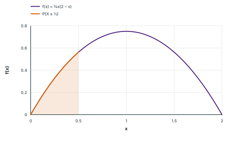
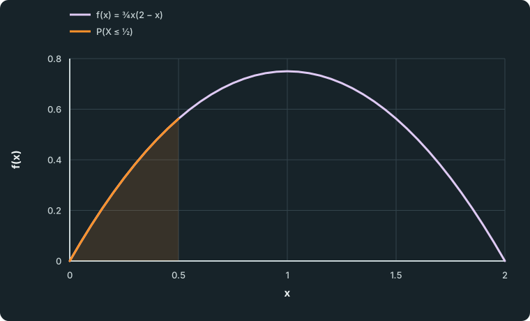
Figure data
This table is included in print while it is open.
| Series | x | f(x) |
|---|---|---|
| f(x) = ¾x(2 − x) | 0.00 | 0.000000 |
| f(x) = ¾x(2 − x) | 0.05 | 0.073125 |
| f(x) = ¾x(2 − x) | 0.10 | 0.142500 |
| f(x) = ¾x(2 − x) | 0.15 | 0.208125 |
| f(x) = ¾x(2 − x) | 0.20 | 0.270000 |
| f(x) = ¾x(2 − x) | 0.25 | 0.328125 |
| f(x) = ¾x(2 − x) | 0.30 | 0.382500 |
| f(x) = ¾x(2 − x) | 0.35 | 0.433125 |
| f(x) = ¾x(2 − x) | 0.40 | 0.480000 |
| f(x) = ¾x(2 − x) | 0.45 | 0.523125 |
| f(x) = ¾x(2 − x) | 0.50 | 0.562500 |
| f(x) = ¾x(2 − x) | 0.55 | 0.598125 |
| f(x) = ¾x(2 − x) | 0.60 | 0.630000 |
| f(x) = ¾x(2 − x) | 0.65 | 0.658125 |
| f(x) = ¾x(2 − x) | 0.70 | 0.682500 |
| f(x) = ¾x(2 − x) | 0.75 | 0.703125 |
| f(x) = ¾x(2 − x) | 0.80 | 0.720000 |
| f(x) = ¾x(2 − x) | 0.85 | 0.733125 |
| f(x) = ¾x(2 − x) | 0.90 | 0.742500 |
| f(x) = ¾x(2 − x) | 0.95 | 0.748125 |
| f(x) = ¾x(2 − x) | 1.00 | 0.750000 |
| f(x) = ¾x(2 − x) | 1.05 | 0.748125 |
| f(x) = ¾x(2 − x) | 1.10 | 0.742500 |
| f(x) = ¾x(2 − x) | 1.15 | 0.733125 |
| f(x) = ¾x(2 − x) | 1.20 | 0.720000 |
| f(x) = ¾x(2 − x) | 1.25 | 0.703125 |
| f(x) = ¾x(2 − x) | 1.30 | 0.682500 |
| f(x) = ¾x(2 − x) | 1.35 | 0.658125 |
| f(x) = ¾x(2 − x) | 1.40 | 0.630000 |
| f(x) = ¾x(2 − x) | 1.45 | 0.598125 |
| f(x) = ¾x(2 − x) | 1.50 | 0.562500 |
| f(x) = ¾x(2 − x) | 1.55 | 0.523125 |
| f(x) = ¾x(2 − x) | 1.60 | 0.480000 |
| f(x) = ¾x(2 − x) | 1.65 | 0.433125 |
| f(x) = ¾x(2 − x) | 1.70 | 0.382500 |
| f(x) = ¾x(2 − x) | 1.75 | 0.328125 |
| f(x) = ¾x(2 − x) | 1.80 | 0.270000 |
| f(x) = ¾x(2 − x) | 1.85 | 0.208125 |
| f(x) = ¾x(2 − x) | 1.90 | 0.142500 |
| f(x) = ¾x(2 − x) | 1.95 | 0.073125 |
| f(x) = ¾x(2 − x) | 2.00 | 0.000000 |
| P(X ≤ ½) | 0.00 | 0.000000 |
| P(X ≤ ½) | 0.05 | 0.073125 |
| P(X ≤ ½) | 0.10 | 0.142500 |
| P(X ≤ ½) | 0.15 | 0.208125 |
| P(X ≤ ½) | 0.20 | 0.270000 |
| P(X ≤ ½) | 0.25 | 0.328125 |
| P(X ≤ ½) | 0.30 | 0.382500 |
| P(X ≤ ½) | 0.35 | 0.433125 |
| P(X ≤ ½) | 0.40 | 0.480000 |
| P(X ≤ ½) | 0.45 | 0.523125 |
| P(X ≤ ½) | 0.50 | 0.562500 |
The height f(x) is not itself a probability. It is probability per unit length: over a short interval of width δ x near x, P ≈ f(x) δ x.
Summaries of a continuous distribution
Replace the sums of the discrete case with integrals over the region where f is non-zero:
| Quantity | Definition |
|---|---|
Mean | E(X) = ∫ x f(x) dx |
Expectation of a function | E(g(X)) = ∫ g(x) f(x) dx |
Variance | Var(X) = E(X²)-[E(X)]² |
Cumulative distribution function | F(x) = P(X ≤ x) = ∫_(-∞)^xf(t) dt, so f(x) = F'(x) where F is differentiable |
Median m | F(m) = 1/2 |
Mode | The value of x where f(x) is greatest |
E(g(X)) is generally not g(E(X)). If the side X of a square is uniform on [0,2], the mean side is 1, but the mean area is E(X²) = ∫₀²(1/2)x² dx = 4/3, not 1².
Worked example 1
A complete density calculation
Worked example 1
A complete density calculation
X has pdf f(x) = kx(2-x) for 0 ≤ x ≤ 2, and 0 otherwise. Find k, E(X), Var(X), the cumulative distribution function F, the median and P(X ≤ 1/2).
Show full solutionHide solution
Make the total probability one
Method
Integrate x(2-x) over [0,2] and set k times it equal to 1.Reason
A pdf must enclose total area 1; this is the only condition that fixes k.Working
Answer
∫₀²x(2-x) dx = [x²-x³/3]₀² = 4/3,; k = 3/4.Mean and variance
Method
The graph is symmetric about x = 1, so E(X) = 1. Find E(X²) by integration.Reason
Symmetry saves one integral, but the variance still needs E(X²).Working
Answer
E(X²) = 3/4∫₀²(2x³-x⁴)dx = (3/4)(8-32/5) = 6/5,; Var(X) = 6/5-1² = 1/5.Cumulative distribution and median
Method
Integrate the pdf from 0 to x, and state F for every real x.Reason
F answers every “at most” question directly, and the median is where F reaches 1/2.Working
Answer
F(x) = { 0, x < 0,; (3/4)x²-(1/4)x³, 0 ≤ x ≤ 2,; 1, x > 2.F(1) = 3/4-1/4 = 1/2, so the median is 1, and
P(X ≤ 1/2) = F(1/2) = 3/16-1/32 = 5/32.
Quick check
F is continuous at both ends: F(0) = 0 and F(2) = 3-2 = 1. The mode is also 1, where the parabola peaks; for a symmetric single-peaked density the mean, median and mode coincide. Writing F for one interval only leaves values of x outside [0,2] undefined.
Densities defined in pieces
When f has different formulas on different intervals, integrate each piece over its own interval and add. The cumulative distribution function then has one formula per piece, and the median lies in whichever piece F crosses 1/2.
Guided practice 1
A skewed density in two pieces
Guided practice 1
A skewed density in two pieces
X has pdf
Find the median and the mean of X, and state the mode.
Try this before viewing the solution
Hint 1
Which piece holds the median?
Find the area of the first piece, ∫₀²(1/3)x dx, and compare it with 1/2.
Hint 2
Two integrals for the mean
E(X) = ∫₀²(1/3)x² dx + ∫₂³(2/3)x(3-x) dx.
Show full solutionHide solution
Locate and find the median
Method
On [0,2], F(x) = (1/6)x², so F(2) = 2/3.Reason
Since 2/3 > 1/2, half the probability is reached inside the first piece.Working
Answer
(1/6)m² = 1/2 ⇒ m = square root of 3 ≈ 1.73,taking the positive root because m lies in [0,2].
Integrate each piece for the mean
Method
Add ∫ x f(x) dx over both intervals.Reason
Each piece contributes its own share of the balance point.Working
Answer
E(X) = ∫₀²x²/3 dx + 2/3∫₂³(3x-x²)dx; = 8/9 + (2/3)[3x²/2-x³/3]₂³; = 8/9 + 2/3 · 7/6 = 8/9 + 7/9 = 5/3 ≈ 1.67.Mode
Working
Answer
f increases to 2/3 at x = 2 and then decreases, so the mode is 2.
Quick check
The mean 1.67 is below the median 1.73, which is below the mode 2. The long left tail on [0,2] pulls the mean furthest from the peak. Checking that the two pieces have areas 2/3 and 1/3 confirms that f is a valid pdf.
Spot the mistake 1
A density bigger than one
Spot the mistake 1
A density bigger than one
Y is uniform on [0,1/2], so its pdf is 2 there. A student says this is impossible because “a probability cannot be 2”, and also that P(Y = 0.25) = 2. Correct both claims.
Write your answer, then compare it with the solution
Show full solutionHide solution
Separate density from probability
Method
A density is probability per unit length; only areas are probabilities.Reason
The total area is 2 × 1/2 = 1, as required.Working
Answer
So a density of 2 is allowed. A single value has zero width, so P(Y = 0.25) = 0; for example P(0.2 ≤ Y ≤ 0.3) = 2 × 0.1 = 0.2.
Common mistake
The claim treats the height of the graph as a probability. The uniform distribution on [a,b] has density 1/(b-a), which exceeds 1 whenever the interval is shorter than 1. Its mean is (a + b)/2 and its variance is ((b-a)²)/12.
Waiting times and the exponential distribution
Suppose events occur as a Poisson process at an average rate of λ per unit time, so the number of events in time t is Po(λ t). The waiting time T until the first event is longer than t exactly when there are no events in [0,t]:
Differentiating F(t) = 1-e^(-λ t) gives the density. This is the exponential distribution T∼Exp(λ):
Solving 1-e^(-λ m) = 1/2 gives the median m = (ln 2)/λ, about 69% of the mean.
An exponential waiting time: median below mean
The density starts at 1 when t = 0 and decreases steadily towards zero, reaching about 0.018 at t = 4. Labels mark the curve at the median t = ln 2 ≈ 0.693, where the density is 0.5, and at the mean t = 1, where the density is about 0.368.
Scroll across to read every label.
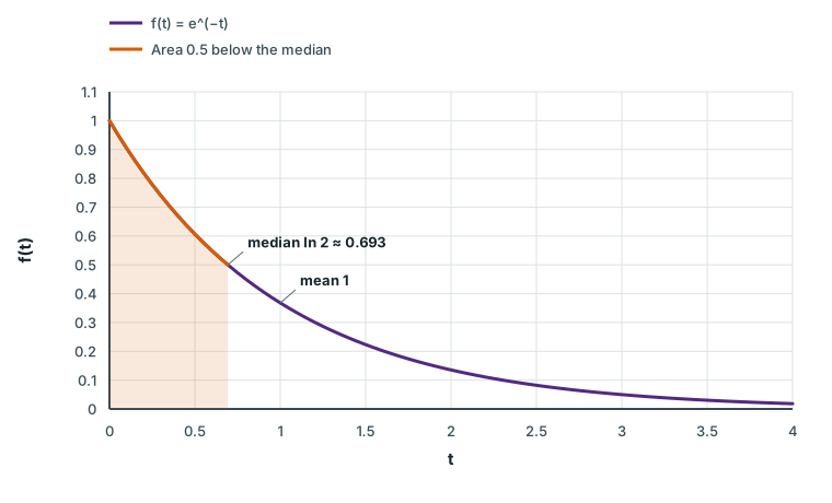
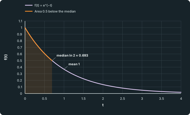
Figure data
This table is included in print while it is open.
| Series | t | f(t) |
|---|---|---|
| f(t) = e^(−t) | 0.000000 | 1.000000 |
| f(t) = e^(−t) | 0.050000 | 0.951229 |
| f(t) = e^(−t) | 0.100000 | 0.904837 |
| f(t) = e^(−t) | 0.150000 | 0.860708 |
| f(t) = e^(−t) | 0.200000 | 0.818731 |
| f(t) = e^(−t) | 0.250000 | 0.778801 |
| f(t) = e^(−t) | 0.300000 | 0.740818 |
| f(t) = e^(−t) | 0.350000 | 0.704688 |
| f(t) = e^(−t) | 0.400000 | 0.670320 |
| f(t) = e^(−t) | 0.450000 | 0.637628 |
| f(t) = e^(−t) | 0.500000 | 0.606531 |
| f(t) = e^(−t) | 0.550000 | 0.576950 |
| f(t) = e^(−t) | 0.600000 | 0.548812 |
| f(t) = e^(−t) | 0.650000 | 0.522046 |
| f(t) = e^(−t) | 0.700000 | 0.496585 |
| f(t) = e^(−t) | 0.750000 | 0.472367 |
| f(t) = e^(−t) | 0.800000 | 0.449329 |
| f(t) = e^(−t) | 0.850000 | 0.427415 |
| f(t) = e^(−t) | 0.900000 | 0.406570 |
| f(t) = e^(−t) | 0.950000 | 0.386741 |
| f(t) = e^(−t) | 1.000000 | 0.367879 |
| f(t) = e^(−t) | 1.050000 | 0.349938 |
| f(t) = e^(−t) | 1.100000 | 0.332871 |
| f(t) = e^(−t) | 1.150000 | 0.316637 |
| f(t) = e^(−t) | 1.200000 | 0.301194 |
| f(t) = e^(−t) | 1.250000 | 0.286505 |
| f(t) = e^(−t) | 1.300000 | 0.272532 |
| f(t) = e^(−t) | 1.350000 | 0.259240 |
| f(t) = e^(−t) | 1.400000 | 0.246597 |
| f(t) = e^(−t) | 1.450000 | 0.234570 |
| f(t) = e^(−t) | 1.500000 | 0.223130 |
| f(t) = e^(−t) | 1.550000 | 0.212248 |
| f(t) = e^(−t) | 1.600000 | 0.201897 |
| f(t) = e^(−t) | 1.650000 | 0.192050 |
| f(t) = e^(−t) | 1.700000 | 0.182684 |
| f(t) = e^(−t) | 1.750000 | 0.173774 |
| f(t) = e^(−t) | 1.800000 | 0.165299 |
| f(t) = e^(−t) | 1.850000 | 0.157237 |
| f(t) = e^(−t) | 1.900000 | 0.149569 |
| f(t) = e^(−t) | 1.950000 | 0.142274 |
| f(t) = e^(−t) | 2.000000 | 0.135335 |
| f(t) = e^(−t) | 2.050000 | 0.128735 |
| f(t) = e^(−t) | 2.100000 | 0.122456 |
| f(t) = e^(−t) | 2.150000 | 0.116484 |
| f(t) = e^(−t) | 2.200000 | 0.110803 |
| f(t) = e^(−t) | 2.250000 | 0.105399 |
| f(t) = e^(−t) | 2.300000 | 0.100259 |
| f(t) = e^(−t) | 2.350000 | 0.095369 |
| f(t) = e^(−t) | 2.400000 | 0.090718 |
| f(t) = e^(−t) | 2.450000 | 0.086294 |
| f(t) = e^(−t) | 2.500000 | 0.082085 |
| f(t) = e^(−t) | 2.550000 | 0.078082 |
| f(t) = e^(−t) | 2.600000 | 0.074274 |
| f(t) = e^(−t) | 2.650000 | 0.070651 |
| f(t) = e^(−t) | 2.700000 | 0.067206 |
| f(t) = e^(−t) | 2.750000 | 0.063928 |
| f(t) = e^(−t) | 2.800000 | 0.060810 |
| f(t) = e^(−t) | 2.850000 | 0.057844 |
| f(t) = e^(−t) | 2.900000 | 0.055023 |
| f(t) = e^(−t) | 2.950000 | 0.052340 |
| f(t) = e^(−t) | 3.000000 | 0.049787 |
| f(t) = e^(−t) | 3.050000 | 0.047359 |
| f(t) = e^(−t) | 3.100000 | 0.045049 |
| f(t) = e^(−t) | 3.150000 | 0.042852 |
| f(t) = e^(−t) | 3.200000 | 0.040762 |
| f(t) = e^(−t) | 3.250000 | 0.038774 |
| f(t) = e^(−t) | 3.300000 | 0.036883 |
| f(t) = e^(−t) | 3.350000 | 0.035084 |
| f(t) = e^(−t) | 3.400000 | 0.033373 |
| f(t) = e^(−t) | 3.450000 | 0.031746 |
| f(t) = e^(−t) | 3.500000 | 0.030197 |
| f(t) = e^(−t) | 3.550000 | 0.028725 |
| f(t) = e^(−t) | 3.600000 | 0.027324 |
| f(t) = e^(−t) | 3.650000 | 0.025991 |
| f(t) = e^(−t) | 3.700000 | 0.024724 |
| f(t) = e^(−t) | 3.750000 | 0.023518 |
| f(t) = e^(−t) | 3.800000 | 0.022371 |
| f(t) = e^(−t) | 3.850000 | 0.021280 |
| f(t) = e^(−t) | 3.900000 | 0.020242 |
| f(t) = e^(−t) | 3.950000 | 0.019255 |
| f(t) = e^(−t) | 4.000000 | 0.018316 |
| Area 0.5 below the median | 0.000000 | 1.000000 |
| Area 0.5 below the median | 0.050000 | 0.951229 |
| Area 0.5 below the median | 0.100000 | 0.904837 |
| Area 0.5 below the median | 0.150000 | 0.860708 |
| Area 0.5 below the median | 0.200000 | 0.818731 |
| Area 0.5 below the median | 0.250000 | 0.778801 |
| Area 0.5 below the median | 0.300000 | 0.740818 |
| Area 0.5 below the median | 0.350000 | 0.704688 |
| Area 0.5 below the median | 0.400000 | 0.670320 |
| Area 0.5 below the median | 0.450000 | 0.637628 |
| Area 0.5 below the median | 0.500000 | 0.606531 |
| Area 0.5 below the median | 0.550000 | 0.576950 |
| Area 0.5 below the median | 0.600000 | 0.548812 |
| Area 0.5 below the median | 0.650000 | 0.522046 |
| Area 0.5 below the median | 0.693147 | 0.500000 |
The exponential distribution is memoryless: having already waited s, the chance of waiting at least t more is the same as at the start,
This suits events that occur at random, such as radioactive decays or calls to a help line. It does not suit lifetimes of parts that wear out, where an old part is more likely to fail soon than a new one.
Check your understanding 1
Waiting for a call
Check your understanding 1
Waiting for a call
Calls arrive as a Poisson process at an average of 3 per hour. Find the probability of waiting more than 30 minutes for the next call, the mean wait, and the median wait in minutes.
Show answerHide answer
With t in hours, T∼Exp(3). Then
which equals the Poisson probability of no calls in 30 minutes. The mean wait is 1/3 hour, 20 minutes, and the median is (ln 2)/3 hour, about 13.9 minutes. The median is less than the mean because the distribution has a long right tail.
Common mistakes
- Reading f(x) as a probability, or writing P(X = a) = f(a).
- Forgetting to state f(x) = 0 or F(x) = 0 and 1 outside the interval.
- Integrating only one piece of a piecewise density, or solving for the median in the wrong piece.
- Writing E(X²) as [E(X)]², or E(g(X)) as g(E(X)).
- Taking the mode as the point where f'(x) = 0 when the greatest density is at an end point.
- Mixing time units: a rate per hour needs times in hours.
Before you move on
Try it yourself 1
How long will the sensor last?
Try it yourself 1
How long will the sensor last?
The time to failure of an electronic sensor is modelled by an exponential distribution with mean 1500 hours.
- Find the probability that a new sensor lasts more than 2000 hours.
- A sensor has already worked for 1000 hours. Find the probability that it lasts at least another 500 hours.
- Find the median lifetime.
Try this before viewing the solution
Show full solutionHide solution
Find the rate
Method
The mean is 1/λ = 1500, so λ = 1/1500 per hour.Reason
The question gives the mean, not the rate; the two are reciprocals.Working
Answer
P(T > 2000) = e^(-2000/1500) = e^(-4/3) ≈ 0.264.Use the memoryless property
Method
P(T > 1500 ∣ T > 1000) = P(T > 500).Reason
The model has no wear: a working sensor is “as good as new”.Working
Answer
P(T > 500) = e^(-500/1500) = e^(-1/3) ≈ 0.717.Median
Working
Answer
m = 1500 ln 2 ≈ 1040 hours.
Quick check
Part 2 is a limitation of the model as well as a calculation: real sensors may wear out, in which case a sensor that has run for 1000 hours would be less likely than a new one to last another 500. A memoryless model is appropriate only if failures happen at random, not through ageing.
Loading reading progress…
Lesson done
- Monday
- Tuesday
- Wednesday
- Thursday
- Friday
- Saturday
- Sunday
Checking learning on this device…
Change goal
Progress options
Loading questions…