On this page
Loading guide controls…
Continue lessonNew guided lessons are not available yet.
Guided lesson options
You stopped at:
ContinueRevision Mode is on. Questions and activities are hidden.
The linked question or activity is hidden by Revision Mode.
Growth models are differential equations: the rate of change of a population depends on the population itself. This lesson solves first-order linear equations with an integrating factor, uses a given substitution to turn a non-linear equation into a linear one, and then reads long-term behaviour from a phase line without solving: equilibria, their stability, the carrying capacity of a logistic model and the effect of harvesting.
The integrating factor
A first-order linear equation has the form
Multiply both sides by the integrating factor I(x) = e^(∫ p(x) dx). Since I' = pI, the left side becomes (d/(dx))(Iy) by the product rule, so
The constant of integration belongs on the right-hand side before you divide by I(x).
Worked example 1
A first-order linear equation
Worked example 1
A first-order linear equation
Solve dy/(dx) + (2/x)y = 3x for x > 0, given that y = 2 when x = 1.
Show full solutionHide solution
Find the integrating factor
Method
p(x) = 2/x, so I = e^(2 ln x) = x².Reason
With x > 0, no modulus is needed in ln x.Working
Answer
Multiplying through: x²dy/(dx) + 2xy = 3x³, that is (d/(dx))(x²y) = 3x³.
Integrate, then fit the condition
Method
x²y = (3/4)x⁴ + C.Reason
Keep C before dividing, so that it is divided by x² too.Working
Answer
At x = 1: 2 = 3/4 + C, so C = 5/4 and
y = 3x²/4 + 5/(4x²).
Quick check
Check: y' = (3/2)x-5/(2x³) and (2/x)y = (3/2)x + 5/(2x³); their sum is 3x. Writing y = (3/4)x² + C (adding C after dividing) would fail this check. The general solution is a family of curves, one for each C; the condition picks one.
Check your understanding 1
Divide only after integrating
Check your understanding 1
Divide only after integrating
Solve dy/(dx)-y/x = x² for x > 0, given that y = 1 when x = 1, and find y when x = 2.
Show answerHide answer
Here p(x) = -1/x, so I = e^(- ln x) = 1/x and
At x = 1, 1 = 1/2 + C, so C = 1/2 and y = (1/2)x³ + (1/2)x. At x = 2, y = 4 + 1 = 5.
A given substitution can make an equation linear
Some equations become linear after a substitution that the question supplies. Differentiate the substitution, replace y and dy/(dx) everywhere, and simplify to a standard form. Remember to return to the original variable. The same idea reduces some second-order equations to the constant-coefficient form.
Check your understanding 2
A logistic-type equation made linear
Check your understanding 2
A logistic-type equation made linear
Use the substitution z = 1/y to find the general solution of dy/(dx) = y-y² for y > 0.
Show answerHide answer
dz/(dx) = -(1/y²)dy/(dx) = -(y-y²)/y² = 1-z, so dz/(dx) + z = 1. With integrating factor e^x: ze^x = e^x + C, so z = 1 + Ce^(-x) and
Every solution with y > 0 tends to 1 as x → ∞.
Phase lines show long-term behaviour
For an equation dP/(dt) = f(P), the equilibria are the values where f(P) = 0. A phase line marks them on a number line and shows, between them, whether P increases (f > 0) or decreases (f < 0). An equilibrium is stable if nearby solutions move towards it, and unstable if they move away. A slope field shows the same information as short line segments with gradient f(P) at many points; it is a sketching aid only.
- Exponential growth: dP/(dt) = kP gives P = P₀e^kt, with no limit for k > 0.
- Logistic growth: dP/(dt) = rP(1-P/K) has equilibria 0 (unstable) and K (stable), the carrying capacity. For r = 1/2, K = 100 and P₀ = 20, the solution is P = 100/(1 + 4e^(-t/2)).
Logistic solutions approach the carrying capacity
Three curves start at P = 20, 60 and 140 when t = 0. The first rises slowly, then steeply around t = 2.8, where it passes 50, then levels off near 100. The second rises and levels off near 100 sooner. The third falls from 140 towards 100. A horizontal reference line marks P = 100.
Scroll across to read every label.
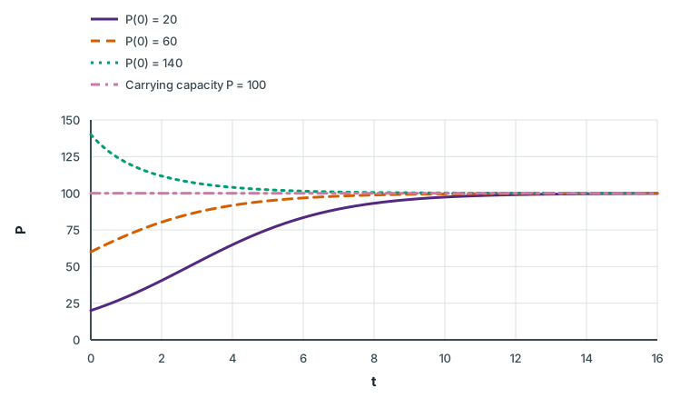
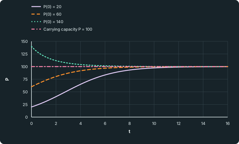
Figure data
This table is included in print while it is open.
| Series | t | P |
|---|---|---|
| P(0) = 20 | 0.00 | 20.0000 |
| P(0) = 20 | 0.25 | 22.0751 |
| P(0) = 20 | 0.50 | 24.3001 |
| P(0) = 20 | 0.75 | 26.6727 |
| P(0) = 20 | 1.00 | 29.1875 |
| P(0) = 20 | 1.25 | 31.8365 |
| P(0) = 20 | 1.50 | 34.6085 |
| P(0) = 20 | 1.75 | 37.4890 |
| P(0) = 20 | 2.00 | 40.4610 |
| P(0) = 20 | 2.25 | 43.5046 |
| P(0) = 20 | 2.50 | 46.5979 |
| P(0) = 20 | 2.75 | 49.7176 |
| P(0) = 20 | 3.00 | 52.8396 |
| P(0) = 20 | 3.25 | 55.9395 |
| P(0) = 20 | 3.50 | 58.9937 |
| P(0) = 20 | 3.75 | 61.9801 |
| P(0) = 20 | 4.00 | 64.8786 |
| P(0) = 20 | 4.25 | 67.6713 |
| P(0) = 20 | 4.50 | 70.3434 |
| P(0) = 20 | 4.75 | 72.8832 |
| P(0) = 20 | 5.00 | 75.2819 |
| P(0) = 20 | 5.25 | 77.5339 |
| P(0) = 20 | 5.50 | 79.6361 |
| P(0) = 20 | 5.75 | 81.5884 |
| P(0) = 20 | 6.00 | 83.3925 |
| P(0) = 20 | 6.25 | 85.0523 |
| P(0) = 20 | 6.50 | 86.5728 |
| P(0) = 20 | 6.75 | 87.9606 |
| P(0) = 20 | 7.00 | 89.2228 |
| P(0) = 20 | 7.25 | 90.3672 |
| P(0) = 20 | 7.50 | 91.4017 |
| P(0) = 20 | 7.75 | 92.3346 |
| P(0) = 20 | 8.00 | 93.1738 |
| P(0) = 20 | 8.25 | 93.9272 |
| P(0) = 20 | 8.50 | 94.6023 |
| P(0) = 20 | 8.75 | 95.2061 |
| P(0) = 20 | 9.00 | 95.7455 |
| P(0) = 20 | 9.25 | 96.2265 |
| P(0) = 20 | 9.50 | 96.6551 |
| P(0) = 20 | 9.75 | 97.0365 |
| P(0) = 20 | 10.00 | 97.3756 |
| P(0) = 20 | 10.25 | 97.6768 |
| P(0) = 20 | 10.50 | 97.9441 |
| P(0) = 20 | 10.75 | 98.1813 |
| P(0) = 20 | 11.00 | 98.3916 |
| P(0) = 20 | 11.25 | 98.5779 |
| P(0) = 20 | 11.50 | 98.7429 |
| P(0) = 20 | 11.75 | 98.8890 |
| P(0) = 20 | 12.00 | 99.0182 |
| P(0) = 20 | 12.25 | 99.1326 |
| P(0) = 20 | 12.50 | 99.2337 |
| P(0) = 20 | 12.75 | 99.3232 |
| P(0) = 20 | 13.00 | 99.4022 |
| P(0) = 20 | 13.25 | 99.4721 |
| P(0) = 20 | 13.50 | 99.5338 |
| P(0) = 20 | 13.75 | 99.5884 |
| P(0) = 20 | 14.00 | 99.6366 |
| P(0) = 20 | 14.25 | 99.6791 |
| P(0) = 20 | 14.50 | 99.7167 |
| P(0) = 20 | 14.75 | 99.7499 |
| P(0) = 20 | 15.00 | 99.7793 |
| P(0) = 20 | 15.25 | 99.8051 |
| P(0) = 20 | 15.50 | 99.8280 |
| P(0) = 20 | 15.75 | 99.8482 |
| P(0) = 20 | 16.00 | 99.8660 |
| P(0) = 60 | 0.00 | 60.0000 |
| P(0) = 60 | 0.25 | 62.9592 |
| P(0) = 60 | 0.50 | 65.8241 |
| P(0) = 60 | 0.75 | 68.5780 |
| P(0) = 60 | 1.00 | 71.2071 |
| P(0) = 60 | 1.25 | 73.7006 |
| P(0) = 60 | 1.50 | 76.0508 |
| P(0) = 60 | 1.75 | 78.2529 |
| P(0) = 60 | 2.00 | 80.3050 |
| P(0) = 60 | 2.25 | 82.2074 |
| P(0) = 60 | 2.50 | 83.9628 |
| P(0) = 60 | 2.75 | 85.5754 |
| P(0) = 60 | 3.00 | 87.0509 |
| P(0) = 60 | 3.25 | 88.3959 |
| P(0) = 60 | 3.50 | 89.6178 |
| P(0) = 60 | 3.75 | 90.7246 |
| P(0) = 60 | 4.00 | 91.7243 |
| P(0) = 60 | 4.25 | 92.6250 |
| P(0) = 60 | 4.50 | 93.4347 |
| P(0) = 60 | 4.75 | 94.1611 |
| P(0) = 60 | 5.00 | 94.8116 |
| P(0) = 60 | 5.25 | 95.3932 |
| P(0) = 60 | 5.50 | 95.9124 |
| P(0) = 60 | 5.75 | 96.3753 |
| P(0) = 60 | 6.00 | 96.7875 |
| P(0) = 60 | 6.25 | 97.1542 |
| P(0) = 60 | 6.50 | 97.4802 |
| P(0) = 60 | 6.75 | 97.7697 |
| P(0) = 60 | 7.00 | 98.0266 |
| P(0) = 60 | 7.25 | 98.2544 |
| P(0) = 60 | 7.50 | 98.4564 |
| P(0) = 60 | 7.75 | 98.6353 |
| P(0) = 60 | 8.00 | 98.7937 |
| P(0) = 60 | 8.25 | 98.9339 |
| P(0) = 60 | 8.50 | 99.0580 |
| P(0) = 60 | 8.75 | 99.1678 |
| P(0) = 60 | 9.00 | 99.2648 |
| P(0) = 60 | 9.25 | 99.3507 |
| P(0) = 60 | 9.50 | 99.4265 |
| P(0) = 60 | 9.75 | 99.4936 |
| P(0) = 60 | 10.00 | 99.5528 |
| P(0) = 60 | 10.25 | 99.6052 |
| P(0) = 60 | 10.50 | 99.6514 |
| P(0) = 60 | 10.75 | 99.6922 |
| P(0) = 60 | 11.00 | 99.7283 |
| P(0) = 60 | 11.25 | 99.7601 |
| P(0) = 60 | 11.50 | 99.7883 |
| P(0) = 60 | 11.75 | 99.8131 |
| P(0) = 60 | 12.00 | 99.8350 |
| P(0) = 60 | 12.25 | 99.8544 |
| P(0) = 60 | 12.50 | 99.8715 |
| P(0) = 60 | 12.75 | 99.8866 |
| P(0) = 60 | 13.00 | 99.8999 |
| P(0) = 60 | 13.25 | 99.9116 |
| P(0) = 60 | 13.50 | 99.9220 |
| P(0) = 60 | 13.75 | 99.9312 |
| P(0) = 60 | 14.00 | 99.9392 |
| P(0) = 60 | 14.25 | 99.9464 |
| P(0) = 60 | 14.50 | 99.9527 |
| P(0) = 60 | 14.75 | 99.9582 |
| P(0) = 60 | 15.00 | 99.9631 |
| P(0) = 60 | 15.25 | 99.9675 |
| P(0) = 60 | 15.50 | 99.9713 |
| P(0) = 60 | 15.75 | 99.9747 |
| P(0) = 60 | 16.00 | 99.9776 |
| P(0) = 140 | 0.00 | 140.0000 |
| P(0) = 140 | 0.25 | 133.7152 |
| P(0) = 140 | 0.50 | 128.6198 |
| P(0) = 140 | 0.75 | 124.4351 |
| P(0) = 140 | 1.00 | 120.9621 |
| P(0) = 140 | 1.25 | 118.0543 |
| P(0) = 140 | 1.50 | 115.6018 |
| P(0) = 140 | 1.75 | 113.5207 |
| P(0) = 140 | 2.00 | 111.7454 |
| P(0) = 140 | 2.25 | 110.2242 |
| P(0) = 140 | 2.50 | 108.9157 |
| P(0) = 140 | 2.75 | 107.7865 |
| P(0) = 140 | 3.00 | 106.8092 |
| P(0) = 140 | 3.25 | 105.9614 |
| P(0) = 140 | 3.50 | 105.2244 |
| P(0) = 140 | 3.75 | 104.5823 |
| P(0) = 140 | 4.00 | 104.0223 |
| P(0) = 140 | 4.25 | 103.5329 |
| P(0) = 140 | 4.50 | 103.1049 |
| P(0) = 140 | 4.75 | 102.7301 |
| P(0) = 140 | 5.00 | 102.4016 |
| P(0) = 140 | 5.25 | 102.1134 |
| P(0) = 140 | 5.50 | 101.8605 |
| P(0) = 140 | 5.75 | 101.6383 |
| P(0) = 140 | 6.00 | 101.4430 |
| P(0) = 140 | 6.25 | 101.2713 |
| P(0) = 140 | 6.50 | 101.1202 |
| P(0) = 140 | 6.75 | 100.9873 |
| P(0) = 140 | 7.00 | 100.8703 |
| P(0) = 140 | 7.25 | 100.7672 |
| P(0) = 140 | 7.50 | 100.6765 |
| P(0) = 140 | 7.75 | 100.5965 |
| P(0) = 140 | 8.00 | 100.5261 |
| P(0) = 140 | 8.25 | 100.4640 |
| P(0) = 140 | 8.50 | 100.4092 |
| P(0) = 140 | 8.75 | 100.3610 |
| P(0) = 140 | 9.00 | 100.3184 |
| P(0) = 140 | 9.25 | 100.2809 |
| P(0) = 140 | 9.50 | 100.2478 |
| P(0) = 140 | 9.75 | 100.2186 |
| P(0) = 140 | 10.00 | 100.1929 |
| P(0) = 140 | 10.25 | 100.1702 |
| P(0) = 140 | 10.50 | 100.1502 |
| P(0) = 140 | 10.75 | 100.1325 |
| P(0) = 140 | 11.00 | 100.1169 |
| P(0) = 140 | 11.25 | 100.1032 |
| P(0) = 140 | 11.50 | 100.0910 |
| P(0) = 140 | 11.75 | 100.0803 |
| P(0) = 140 | 12.00 | 100.0709 |
| P(0) = 140 | 12.25 | 100.0625 |
| P(0) = 140 | 12.50 | 100.0552 |
| P(0) = 140 | 12.75 | 100.0487 |
| P(0) = 140 | 13.00 | 100.0430 |
| P(0) = 140 | 13.25 | 100.0379 |
| P(0) = 140 | 13.50 | 100.0335 |
| P(0) = 140 | 13.75 | 100.0295 |
| P(0) = 140 | 14.00 | 100.0261 |
| P(0) = 140 | 14.25 | 100.0230 |
| P(0) = 140 | 14.50 | 100.0203 |
| P(0) = 140 | 14.75 | 100.0179 |
| P(0) = 140 | 15.00 | 100.0158 |
| P(0) = 140 | 15.25 | 100.0139 |
| P(0) = 140 | 15.50 | 100.0123 |
| P(0) = 140 | 15.75 | 100.0109 |
| P(0) = 140 | 16.00 | 100.0096 |
| Carrying capacity P = 100 | 0.00 | 100.0000 |
| Carrying capacity P = 100 | 16.00 | 100.0000 |
Common mistakes
- Using e^(∫ q(x) dx), or forgetting the integral, when forming the integrating factor e^(∫ p(x) dx).
- Applying the integrating factor before writing the equation in the form dy/(dx) + p(x)y = q(x).
- Adding the constant after dividing by the integrating factor.
- Differentiating a substitution such as z = 1/y without the chain rule: dz/(dx) = -(1/y²)dy/(dx).
- Calling an equilibrium stable without checking the sign of dP/(dt) on both sides of it.
Before you move on
Try it yourself 1
Harvesting a fish population
Try it yourself 1
Harvesting a fish population
A fish population (in thousands) is modelled by
where 12 thousand fish are harvested per year. Find the equilibria and their stability, and describe what happens if P(0) = 30 and if P(0) = 50. What is the largest constant harvest that still allows an equilibrium?
Write your answer, then compare it with the solution
Hint 1
Clear the fractions
Multiplying f(P) = 0 by -200 gives P²-100P + 2400 = 0.
Show full solutionHide solution
Equilibria and stability
Method
P²-100P + 2400 = (P-40)(P-60) = 0.Reason
f is a downward parabola in P, so it is positive only between its roots.Working
Answer
f < 0 for P < 40, f > 0 for 40 < P < 60 and f < 0 for P > 60. So 40 is unstable and 60 is stable.
Read the two starting values
Method
Follow the arrows of the phase line.Reason
Solutions cannot cross an equilibrium.Working
Answer
From 30, P decreases and the population collapses: the model reaches 0 in finite time. From 50, P increases towards 60 thousand.
The largest sustainable harvest
Method
An equilibrium needs (1/2)P(1-P/100) = h to have a root.Reason
The left side is greatest at P = 50, where it equals 12.5.Working
Answer
So the largest constant harvest is 12.5 thousand fish per year. Any larger harvest makes dP/(dt) < 0 for every P.
Quick check
Harvesting at 12 turns the unharvested unstable equilibrium 0 into an unstable threshold at 40: a population below it is lost. The threshold is the practical lesson: a harvest that is safe for a large population can drive a smaller one to extinction.
Loading reading progress…
Lesson done
- Monday
- Tuesday
- Wednesday
- Thursday
- Friday
- Saturday
- Sunday
Checking learning on this device…
Change goal
Progress options
Loading questions…