On this page
Loading guide controls…
Continue lessonNew guided lessons are not available yet.
Guided lesson options
You stopped at:
ContinueRevision Mode is on. Questions and activities are hidden.
The linked question or activity is hidden by Revision Mode.
The height of a hillside depends on two coordinates, and so does the cost of a box with two adjustable sides. A function z = f(x,y) is a surface above the xy-plane, and the calculus of one variable extends to it one direction at a time. This lesson shows how to differentiate with one variable held fixed, how the two partial derivatives combine into a gradient, tangent plane and linear approximation, and how second derivatives classify the flat points of a surface as maxima, minima or saddles.
Differentiate with one variable fixed
The partial derivative fₓ = (∂ f)/(∂ x) is the gradient of the surface in the x-direction: differentiate with respect to x, treating y as a constant. Likewise fy treats x as a constant. Differentiating again gives the second-order partial derivatives fₓₓ, f_yy and the mixed derivatives f_xy and f_yx, which are equal for every function in this course.
For f(x,y) = x²y + y³,
All the one-variable rules still apply. In x²e^y, the factor e^y is a constant when you differentiate with respect to x; in sin(xy), the chain rule gives fₓ = y cos(xy).
Two directions through one surface point
The solid section is f(1 + s, 1) = (1 + s)² + 1. The dashed section is f(1, 1 + s) = 1 + s + (1 + s)³. Both have height 2 at s = 0, with different slopes there.
Scroll across to read every label.
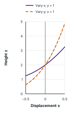
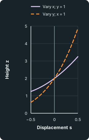
Figure data
This table is included in print while it is open.
| Displacement s | Vary x; y = 1 | Vary y; x = 1 |
|---|---|---|
| -0.500 | 1.250000 | 0.6250 |
| -0.475 | 1.275625 | 0.6697 |
| -0.450 | 1.302500 | 0.7164 |
| -0.425 | 1.330625 | 0.7651 |
| -0.400 | 1.360000 | 0.8160 |
| -0.375 | 1.390625 | 0.8691 |
| -0.350 | 1.422500 | 0.9246 |
| -0.325 | 1.455625 | 0.9825 |
| -0.300 | 1.490000 | 1.0430 |
| -0.275 | 1.525625 | 1.1061 |
| -0.250 | 1.562500 | 1.1719 |
| -0.225 | 1.600625 | 1.2405 |
| -0.200 | 1.640000 | 1.3120 |
| -0.175 | 1.680625 | 1.3865 |
| -0.150 | 1.722500 | 1.4641 |
| -0.125 | 1.765625 | 1.5449 |
| -0.100 | 1.810000 | 1.6290 |
| -0.075 | 1.855625 | 1.7165 |
| -0.050 | 1.902500 | 1.8074 |
| -0.025 | 1.950625 | 1.9019 |
| 0.000 | 2.000000 | 2.0000 |
| 0.025 | 2.050625 | 2.1019 |
| 0.050 | 2.102500 | 2.2076 |
| 0.075 | 2.155625 | 2.3173 |
| 0.100 | 2.210000 | 2.4310 |
| 0.125 | 2.265625 | 2.5488 |
| 0.150 | 2.322500 | 2.6709 |
| 0.175 | 2.380625 | 2.7972 |
| 0.200 | 2.440000 | 2.9280 |
| 0.225 | 2.500625 | 3.0633 |
| 0.250 | 2.562500 | 3.2031 |
| 0.275 | 2.625625 | 3.3477 |
| 0.300 | 2.690000 | 3.4970 |
| 0.325 | 2.755625 | 3.6512 |
| 0.350 | 2.822500 | 3.8104 |
| 0.375 | 2.890625 | 3.9746 |
| 0.400 | 2.960000 | 4.1440 |
| 0.425 | 3.030625 | 4.3186 |
| 0.450 | 3.102500 | 4.4986 |
| 0.475 | 3.175625 | 4.6840 |
| 0.500 | 3.250000 | 4.8750 |
Check your understanding 1
Hold the other variable still
Check your understanding 1
Hold the other variable still
For f(x,y) = x²e^y + 3xy², find fₓ, fy and f_xy, and evaluate each at (1,0).
Show answerHide answer
Differentiating fy with respect to x gives the same 2xe^y + 6y.
Gradient, tangent plane and linear approximation
The two partial derivatives form the gradient vector, which points in the direction of steepest increase. The rate of change in the direction of a unit vector u is the directional derivative:
Since ∇ f · u = |∇ f| cos θ, the directional derivative is greatest, equal to |∇ f|, when u points along ∇ f, and zero along a contour, perpendicular to ∇ f.
Close to a point (a,b), a smooth surface is almost flat. Its tangent plane there is
and using this plane to estimate nearby values is local linearisation. A normal vector to the surface z = f(x,y) at the point is (fₓ; fy; -1).
Worked example 1
Tangent plane and normal line to a dome
Worked example 1
Tangent plane and normal line to a dome
Find the equation of the tangent plane and a vector equation of the normal line to the surface z = 4-x²-2y² at the point (1,1,1).
Show full solutionHide solution
Evaluate the partial derivatives
Method
fₓ = -2x and fy = -4y, so fₓ(1,1) = -2 and fy(1,1) = -4.Reason
These are the slopes of the plane in the x- and y-directions. First check that the point lies on the surface: 4-1-2 = 1.Working
Answer
z = 1-2(x-1)-4(y-1),; 2x + 4y + z = 7.Use the normal vector
Working
Answer
A normal is (fₓ,fy,-1) = (-2,-4,-1), or equivalently (2,4,1), which matches the coefficients of the plane. The normal line is
r = (1; 1; 1) + t (2; 4; 1).
Quick check
Substituting (1,1,1) into 2x + 4y + z gives 7, so the plane passes through the point. The normal line connects this lesson to the vector equations of lines and planes from H2 Mathematics.
Check your understanding 2
Rates and estimates at a point
Check your understanding 2
Rates and estimates at a point
For f(x,y) = x²y + y³ at (1,2): find ∇ f, the directional derivative in the direction of (3,4), and the greatest rate of increase. Use the tangent plane to estimate f(1.1,1.9) and compare with the exact value.
Show answerHide answer
∇ f(1,2) = (4,13). The direction (3,4) has length 5, so u = (1/5)(3,4) and
The greatest rate of increase is |∇ f| = square root of (4² + 13²) = square root of 185 ≈ 13.6.
Since f(1,2) = 10, the tangent plane gives
The exact value is 1.21 × 1.9 + 1.9³ = 9.158; the small difference comes from the curvature that the plane ignores.
Stationary points and the second-derivative test
At a stationary point both fₓ = 0 and fy = 0, so the tangent plane is horizontal. Unlike a curve, a surface can be flat at a point that is neither a maximum nor a minimum: at a saddle point it rises in some directions and falls in others. Classify a stationary point with
evaluated at the point:
| Condition at the stationary point | Nature |
|---|---|
| D > 0 and fₓₓ > 0 | local minimum |
| D > 0 and fₓₓ < 0 | local maximum |
| D < 0 | saddle point |
| D = 0 | test inconclusive |
The test comes from the quadratic approximation near a stationary point (a,b), where the linear terms vanish:
Completing the square shows that the bracket keeps one sign for every small (h,k) ≠ (0,0) exactly when D > 0, with the sign of fₓₓ; when D < 0 it takes both signs.
Worked example 2
A minimum and a saddle
Worked example 2
A minimum and a saddle
Find and classify the stationary points of f(x,y) = x³-3x + y²-4y.
Show full solutionHide solution
Solve both equations
Method
fₓ = 3x²-3 = 0 and fy = 2y-4 = 0.Reason
A stationary point needs both partial derivatives zero at once.Working
Answer
x = ±1 and y = 2, so the stationary points are (1,2) and (-1,2).
Apply the test
Method
fₓₓ = 6x, f_yy = 2, f_xy = 0, so D = 12x.Reason
The sign of D separates extrema from saddles.Working
Answer
At (1,2), D = 12 > 0 and fₓₓ = 6 > 0: a local minimum, with f(1,2) = -6.
At (-1,2), D = -12 < 0: a saddle point, with f(-1,2) = -2.
Quick check
At the saddle, moving in x from (-1,2) decreases f, because x³-3x has a maximum at x = -1, while moving in y increases it. The figure below shows both sections. A local minimum need not be a global one: f → -∞ as x → -∞.
Two sections through the saddle point (−1, 2)
The horizontal axis is the distance s moved from (−1, 2). The solid curve f(−1 + s, 2) = s³ − 3s² − 2 rises to −2 at s = 0 and falls on both sides near it, reaching −6 at s = −1 and −4 at s = 1. The dashed curve f(−1, 2 + s) = s² − 2 dips to −2 at s = 0 and rises to −1 at s = ±1. The two curves touch at (0, −2).
Scroll across to read every label.
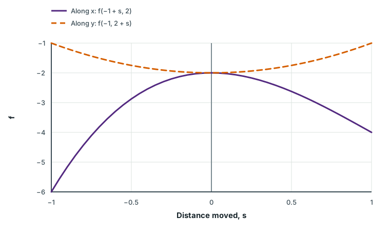
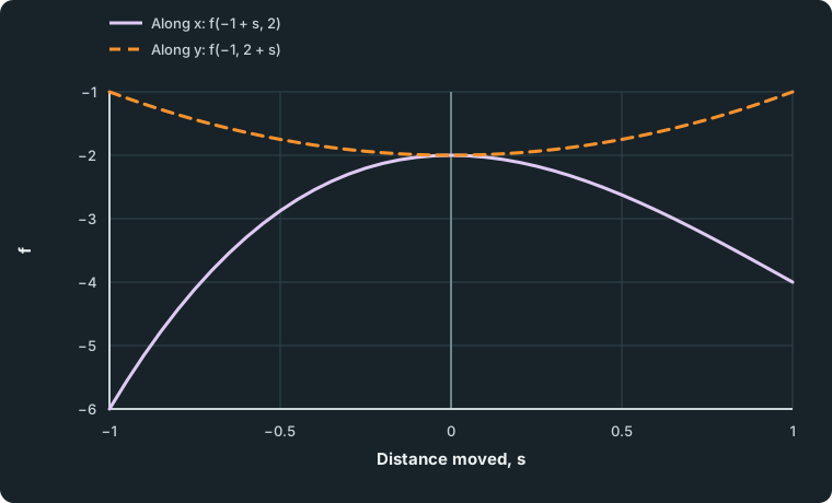
Figure data
This table is included in print while it is open.
| Distance moved, s | Along x: f(−1 + s, 2) | Along y: f(−1, 2 + s) |
|---|---|---|
| -1.00 | -6.000000 | -1.0000 |
| -0.95 | -5.564875 | -1.0975 |
| -0.90 | -5.159000 | -1.1900 |
| -0.85 | -4.781625 | -1.2775 |
| -0.80 | -4.432000 | -1.3600 |
| -0.75 | -4.109375 | -1.4375 |
| -0.70 | -3.813000 | -1.5100 |
| -0.65 | -3.542125 | -1.5775 |
| -0.60 | -3.296000 | -1.6400 |
| -0.55 | -3.073875 | -1.6975 |
| -0.50 | -2.875000 | -1.7500 |
| -0.45 | -2.698625 | -1.7975 |
| -0.40 | -2.544000 | -1.8400 |
| -0.35 | -2.410375 | -1.8775 |
| -0.30 | -2.297000 | -1.9100 |
| -0.25 | -2.203125 | -1.9375 |
| -0.20 | -2.128000 | -1.9600 |
| -0.15 | -2.070875 | -1.9775 |
| -0.10 | -2.031000 | -1.9900 |
| -0.05 | -2.007625 | -1.9975 |
| 0.00 | -2.000000 | -2.0000 |
| 0.05 | -2.007375 | -1.9975 |
| 0.10 | -2.029000 | -1.9900 |
| 0.15 | -2.064125 | -1.9775 |
| 0.20 | -2.112000 | -1.9600 |
| 0.25 | -2.171875 | -1.9375 |
| 0.30 | -2.243000 | -1.9100 |
| 0.35 | -2.324625 | -1.8775 |
| 0.40 | -2.416000 | -1.8400 |
| 0.45 | -2.516375 | -1.7975 |
| 0.50 | -2.625000 | -1.7500 |
| 0.55 | -2.741125 | -1.6975 |
| 0.60 | -2.864000 | -1.6400 |
| 0.65 | -2.992875 | -1.5775 |
| 0.70 | -3.127000 | -1.5100 |
| 0.75 | -3.265625 | -1.4375 |
| 0.80 | -3.408000 | -1.3600 |
| 0.85 | -3.553375 | -1.2775 |
| 0.90 | -3.701000 | -1.1900 |
| 0.95 | -3.850125 | -1.0975 |
| 1.00 | -4.000000 | -1.0000 |
Spot the mistake 1
Positive in both directions, still a saddle
Spot the mistake 1
Positive in both directions, still a saddle
A student says that f(x,y) = x² + 3xy + y² has a minimum at the origin because fₓₓ = 2 > 0 and f_yy = 2 > 0. Explain the error.
Write your answer, then compare it with the solution
Show full solutionHide solution
Include the mixed derivative
Method
f_xy = 3, so D = 2 × 2-3² = -5 < 0.Reason
fₓₓ and f_yy only describe the two axis directions.Working
Answer
The origin is a saddle point. Along the line y = -x, f = x²-3x² + x² = -x² < 0 for x ≠ 0, while along the axes f > 0.
Common mistake
Always compute D with the mixed derivative. A single line along which f falls below its stationary value is enough to rule out a minimum.
Common mistakes
- Treating the other variable as zero instead of as a constant: in (∂/(∂ x))(x²y), the answer is 2xy, not 2x or 0.
- Using a non-unit direction vector in Dᵤf = ∇ f · u.
- Solving fₓ = 0 and fy = 0 separately and combining every x with every y, instead of solving them simultaneously.
- Classifying with fₓₓ and f_yy alone and ignoring f_xy.
- Concluding “minimum” or “maximum” when D = 0. The test gives no information there.
Before you move on
Try it yourself 1
Two stationary points linked together
Try it yourself 1
Two stationary points linked together
Find and classify the stationary points of f(x,y) = x³ + y³-3xy.
Try this before viewing the solution
Show full solutionHide solution
Solve the equations together
Method
fₓ = 3x²-3y = 0 and fy = 3y²-3x = 0 give y = x² and x = y².Reason
Each equation contains both variables, so substitute one into the other.Working
Answer
x = (x²)² = x⁴,; x(x³-1) = 0,so the real solutions are x = 0 and x = 1, giving the points (0,0) and (1,1).
Classify both points
Working
Answer
fₓₓ = 6x, f_yy = 6y and f_xy = -3, so D = 36xy-9.
At (0,0), D = -9 < 0: a saddle point.
At (1,1), D = 27 > 0 and fₓₓ = 6 > 0: a local minimum, with f(1,1) = 1 + 1-3 = -1.
Quick check
At the origin, fₓₓ = f_yy = 0, so the pure second derivatives say nothing; the mixed term alone makes D negative. Along y = x near the origin, f = 2x³-3x² < 0 for small x ≠ 0, while along y = -x, f = 3x² > 0: the surface falls one way and rises the other.
Loading reading progress…
Lesson done
- Monday
- Tuesday
- Wednesday
- Thursday
- Friday
- Saturday
- Sunday
Checking learning on this device…
Change goal
Progress options
Loading questions…