On this page
Loading guide controls…
Continue lessonNew guided lessons are not available yet.
Guided lesson options
You stopped at:
ContinueRevision Mode is on. Questions and activities are hidden.
The linked question or activity is hidden by Revision Mode.
Is a die fair? Do call arrivals follow a Poisson model? Is subject choice linked to school? Each question compares counts observed in categories with the counts a model predicts. The χ² test turns all the category-by-category discrepancies into one number and asks whether it is too large to be put down to chance. This lesson builds that statistic, explains where its degrees of freedom come from, and then applies it to goodness-of-fit tests and to contingency tables, including the pooling and interpretation steps that examiners look for.
Comparing observed and expected frequencies
For each category, compare the observed frequency O with the frequency E expected if the null hypothesis H₀ is true. Squaring stops positive and negative discrepancies cancelling, and dividing by E judges each discrepancy relative to its size: being 5 out when 10 was expected matters far more than being 5 out when 1000 was expected.
If H₀ is true and every expected frequency is at least 5, X² approximately follows a χ² distribution with ν degrees of freedom. Small values mean the data agree with the model; large values are evidence against it. The test is therefore always upper-tailed: reject H₀ when X² exceeds the critical value χ²ν at the chosen level, or equivalently when the p-value P(χ²ν ≥ X²) is less than the significance level.
Where a χ² statistic falls against the critical value
A right-skewed density curve starts at 0 when x = 0, peaks at about 0.154 when x = 3 and falls towards zero by x = 20. The area to the right of x = 11.07 is shaded. A vertical marker at x = 4.5, the die statistic, lies to the left of the shaded region, where the density is about 0.13.
Scroll across to read every label.
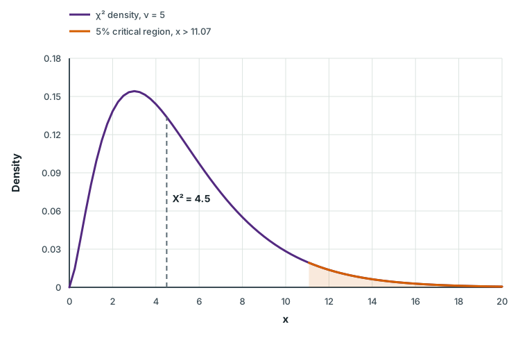
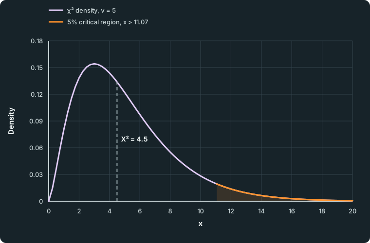
Figure data
This table is included in print while it is open.
| Series | x | Density |
|---|---|---|
| χ² density, ν = 5 | 0.0000 | 0.000000 |
| χ² density, ν = 5 | 0.2500 | 0.014669 |
| χ² density, ν = 5 | 0.5000 | 0.036616 |
| χ² density, ν = 5 | 0.7500 | 0.059364 |
| χ² density, ν = 5 | 1.0000 | 0.080657 |
| χ² density, ν = 5 | 1.2500 | 0.099476 |
| χ² density, ν = 5 | 1.5000 | 0.115400 |
| χ² density, ν = 5 | 1.7500 | 0.128333 |
| χ² density, ν = 5 | 2.0000 | 0.138369 |
| χ² density, ν = 5 | 2.2500 | 0.145707 |
| χ² density, ν = 5 | 2.5000 | 0.150602 |
| χ² density, ν = 5 | 2.7500 | 0.153332 |
| χ² density, ν = 5 | 3.0000 | 0.154180 |
| χ² density, ν = 5 | 3.2500 | 0.153421 |
| χ² density, ν = 5 | 3.5000 | 0.151313 |
| χ² density, ν = 5 | 3.7500 | 0.148093 |
| χ² density, ν = 5 | 4.0000 | 0.143976 |
| χ² density, ν = 5 | 4.2500 | 0.139154 |
| χ² density, ν = 5 | 4.5000 | 0.133797 |
| χ² density, ν = 5 | 4.7500 | 0.128050 |
| χ² density, ν = 5 | 5.0000 | 0.122042 |
| χ² density, ν = 5 | 5.2500 | 0.115879 |
| χ² density, ν = 5 | 5.5000 | 0.109654 |
| χ² density, ν = 5 | 5.7500 | 0.103441 |
| χ² density, ν = 5 | 6.0000 | 0.097304 |
| χ² density, ν = 5 | 6.2500 | 0.091293 |
| χ² density, ν = 5 | 6.5000 | 0.085448 |
| χ² density, ν = 5 | 6.7500 | 0.079800 |
| χ² density, ν = 5 | 7.0000 | 0.074371 |
| χ² density, ν = 5 | 7.2500 | 0.069180 |
| χ² density, ν = 5 | 7.5000 | 0.064236 |
| χ² density, ν = 5 | 7.7500 | 0.059546 |
| χ² density, ν = 5 | 8.0000 | 0.055112 |
| χ² density, ν = 5 | 8.2500 | 0.050934 |
| χ² density, ν = 5 | 8.5000 | 0.047007 |
| χ² density, ν = 5 | 8.7500 | 0.043327 |
| χ² density, ν = 5 | 9.0000 | 0.039887 |
| χ² density, ν = 5 | 9.2500 | 0.036677 |
| χ² density, ν = 5 | 9.5000 | 0.033688 |
| χ² density, ν = 5 | 9.7500 | 0.030911 |
| χ² density, ν = 5 | 10.0000 | 0.028335 |
| χ² density, ν = 5 | 10.2500 | 0.025949 |
| χ² density, ν = 5 | 10.5000 | 0.023743 |
| χ² density, ν = 5 | 10.7500 | 0.021705 |
| χ² density, ν = 5 | 11.0000 | 0.019827 |
| χ² density, ν = 5 | 11.2500 | 0.018097 |
| χ² density, ν = 5 | 11.5000 | 0.016506 |
| χ² density, ν = 5 | 11.7500 | 0.015044 |
| χ² density, ν = 5 | 12.0000 | 0.013702 |
| χ² density, ν = 5 | 12.2500 | 0.012472 |
| χ² density, ν = 5 | 12.5000 | 0.011345 |
| χ² density, ν = 5 | 12.7500 | 0.010314 |
| χ² density, ν = 5 | 13.0000 | 0.009371 |
| χ² density, ν = 5 | 13.2500 | 0.008510 |
| χ² density, ν = 5 | 13.5000 | 0.007723 |
| χ² density, ν = 5 | 13.7500 | 0.007006 |
| χ² density, ν = 5 | 14.0000 | 0.006352 |
| χ² density, ν = 5 | 14.2500 | 0.005757 |
| χ² density, ν = 5 | 14.5000 | 0.005214 |
| χ² density, ν = 5 | 14.7500 | 0.004721 |
| χ² density, ν = 5 | 15.0000 | 0.004273 |
| χ² density, ν = 5 | 15.2500 | 0.003865 |
| χ² density, ν = 5 | 15.5000 | 0.003495 |
| χ² density, ν = 5 | 15.7500 | 0.003160 |
| χ² density, ν = 5 | 16.0000 | 0.002855 |
| χ² density, ν = 5 | 16.2500 | 0.002579 |
| χ² density, ν = 5 | 16.5000 | 0.002329 |
| χ² density, ν = 5 | 16.7500 | 0.002102 |
| χ² density, ν = 5 | 17.0000 | 0.001897 |
| χ² density, ν = 5 | 17.2500 | 0.001711 |
| χ² density, ν = 5 | 17.5000 | 0.001543 |
| χ² density, ν = 5 | 17.7500 | 0.001391 |
| χ² density, ν = 5 | 18.0000 | 0.001253 |
| χ² density, ν = 5 | 18.2500 | 0.001129 |
| χ² density, ν = 5 | 18.5000 | 0.001017 |
| χ² density, ν = 5 | 18.7500 | 0.000916 |
| χ² density, ν = 5 | 19.0000 | 0.000824 |
| χ² density, ν = 5 | 19.2500 | 0.000742 |
| χ² density, ν = 5 | 19.5000 | 0.000668 |
| χ² density, ν = 5 | 19.7500 | 0.000600 |
| χ² density, ν = 5 | 20.0000 | 0.000540 |
| 5% critical region, x > 11.07 | 11.0705 | 0.019325 |
| 5% critical region, x > 11.07 | 11.2500 | 0.018097 |
| 5% critical region, x > 11.07 | 11.5000 | 0.016506 |
| 5% critical region, x > 11.07 | 11.7500 | 0.015044 |
| 5% critical region, x > 11.07 | 12.0000 | 0.013702 |
| 5% critical region, x > 11.07 | 12.2500 | 0.012472 |
| 5% critical region, x > 11.07 | 12.5000 | 0.011345 |
| 5% critical region, x > 11.07 | 12.7500 | 0.010314 |
| 5% critical region, x > 11.07 | 13.0000 | 0.009371 |
| 5% critical region, x > 11.07 | 13.2500 | 0.008510 |
| 5% critical region, x > 11.07 | 13.5000 | 0.007723 |
| 5% critical region, x > 11.07 | 13.7500 | 0.007006 |
| 5% critical region, x > 11.07 | 14.0000 | 0.006352 |
| 5% critical region, x > 11.07 | 14.2500 | 0.005757 |
| 5% critical region, x > 11.07 | 14.5000 | 0.005214 |
| 5% critical region, x > 11.07 | 14.7500 | 0.004721 |
| 5% critical region, x > 11.07 | 15.0000 | 0.004273 |
| 5% critical region, x > 11.07 | 15.2500 | 0.003865 |
| 5% critical region, x > 11.07 | 15.5000 | 0.003495 |
| 5% critical region, x > 11.07 | 15.7500 | 0.003160 |
| 5% critical region, x > 11.07 | 16.0000 | 0.002855 |
| 5% critical region, x > 11.07 | 16.2500 | 0.002579 |
| 5% critical region, x > 11.07 | 16.5000 | 0.002329 |
| 5% critical region, x > 11.07 | 16.7500 | 0.002102 |
| 5% critical region, x > 11.07 | 17.0000 | 0.001897 |
| 5% critical region, x > 11.07 | 17.2500 | 0.001711 |
| 5% critical region, x > 11.07 | 17.5000 | 0.001543 |
| 5% critical region, x > 11.07 | 17.7500 | 0.001391 |
| 5% critical region, x > 11.07 | 18.0000 | 0.001253 |
| 5% critical region, x > 11.07 | 18.2500 | 0.001129 |
| 5% critical region, x > 11.07 | 18.5000 | 0.001017 |
| 5% critical region, x > 11.07 | 18.7500 | 0.000916 |
| 5% critical region, x > 11.07 | 19.0000 | 0.000824 |
| 5% critical region, x > 11.07 | 19.2500 | 0.000742 |
| 5% critical region, x > 11.07 | 19.5000 | 0.000668 |
| 5% critical region, x > 11.07 | 19.7500 | 0.000600 |
| 5% critical region, x > 11.07 | 20.0000 | 0.000540 |
Degrees of freedom count free categories
ν is the number of categories whose frequencies are free to vary once the constraints are imposed. The expected frequencies are always scaled to the same total as the observed ones, which removes one degree of freedom. Each parameter estimated from the data removes another:
| Test | Degrees of freedom |
|---|---|
Goodness of fit, k classes after pooling, m parameters estimated from the data | ν = k-1-m |
Independence in an r × c contingency table | ν = (r-1)(c-1) |
Count classes after any pooling. If an expected frequency is below 5, combine that class with a neighbour, adding both the observed and the expected frequencies, before you compute X².
Worked example 1
Is the die fair?
Worked example 1
Is the die fair?
A die is rolled 120 times, with these results:
| Score | 1 | 2 | 3 | 4 | 5 | 6 |
|---|---|---|---|---|---|---|
| Frequency | 15 | 25 | 18 | 22 | 16 | 24 |
Test at the 5% level of significance whether the die is fair.
Show full solutionHide solution
State the hypotheses and expected frequencies
Method
H₀: the die is fair. H₁: the die is not fair. Under H₀ each score has expected frequency 120 × 1/6 = 20.Reason
Hypotheses are statements about the population (the die), not about this sample. All six expected frequencies are at least 5, so no pooling is needed.Working
Answer
The differences O-E are -5, 5, -2, 2, -4, 4.
Compute the statistic
Method
Square each difference, divide by E, and add.Reason
Every E is 20, so the division can be done once at the end.Working
Answer
X² = (25 + 25 + 4 + 4 + 16 + 16)/20; = 4.5.Compare and conclude in context
Method
ν = 6-1 = 5, and the 5% critical value is χ²₅(0.05) = 11.07.Reason
Only the total constrains the expected frequencies; no parameter was estimated from the data.Working
Answer
Since 4.5 < 11.07 (equivalently, p = P(χ²₅ ≥ 4.5) ≈ 0.480 > 0.05), do not reject H₀. There is insufficient evidence at the 5% level to conclude that the die is not fair.
Quick check
Not rejecting H₀ does not prove the die is fair: it says these 120 rolls are consistent with fairness. A biased die can easily produce data like these in a small sample.
Fitting a model with an estimated parameter
When the model has a parameter you do not know, estimate it from the same data. That estimate makes the expected frequencies agree more closely with the observations, so it costs one degree of freedom.
Worked example 2
Do emails arrive at random?
Worked example 2
Do emails arrive at random?
The number of emails arriving at a help desk is recorded for 120 five-minute intervals. No interval had more than 5 emails.
| Emails | 0 | 1 | 2 | 3 | 4 | 5 |
|---|---|---|---|---|---|---|
| Intervals | 30 | 37 | 29 | 14 | 7 | 3 |
Test at the 5% level whether a Poisson distribution is a suitable model.
Show full solutionHide solution
Estimate the mean
Method
H₀: the number of emails in a five-minute interval follows a Poisson distribution. H₁: it does not.Reason
The hypothesis names a Poisson model but not its mean, so the sample mean estimates λ.Working
Answer
λ hat = (0(30) + 1(37) + 2(29) + 3(14) + 4(7) + 5(3))/120; = 180/120 = 1.5.Find the expected frequencies and pool
Method
Multiply each Poisson probability by 120. The last class must cover every value from 4 upwards.Reason
The model allows 5,6,7,… emails even though none were observed above 5, so the final expected frequency uses P(X ≥ 4), not P(X = 4).Working
Answer
With X∼Po(1.5), the expected frequencies are 26.78, 40.16, 30.12, 15.06 for 0 to 3, then 5.65 for exactly 4 and 2.23 for 5 or more. The last is below 5, so combine 4 and 5 or more into one class “4 or more”, with O = 7 + 3 = 10 and E = 7.88.
Emails 0 1 2 3 ≥ 4 O 30 37 29 14 10 E 26.78 40.16 30.12 15.06 7.88 Test with the reduced degrees of freedom
Method
ν = 5-1-1 = 3: five classes after pooling, one for the total and one for λ hat.Reason
Counting the six original classes, or forgetting the estimated mean, would use the wrong critical value.Working
Answer
X² = 0.388 + 0.249 + 0.042 + 0.075 + 0.572; ≈ 1.33.The 5% critical value is χ²₃(0.05) = 7.815. Since 1.33 < 7.815 (p ≈ 0.72), do not reject H₀. There is insufficient evidence at the 5% level to say that a Poisson model is unsuitable; the arrivals are consistent with emails arriving at random at a constant average rate.
Quick check
Keep the expected frequencies to at least two decimal places; they are not counts and need not be whole numbers. A check: the expected frequencies add to 120, the same as the observed total.
Spot the mistake 1
A spinner tested with percentages
Spot the mistake 1
A spinner tested with percentages
A three-colour spinner is spun 60 times and lands on red 26 times, blue 20 times and green 14 times. A student converts these to percentages, 43.3%, 33.3% and 23.3%, compares them with 33.3% each and finds X² = 6.0. As 6.0 > 5.991, the student concludes at the 5% level that the spinner is biased. Explain the error and give the correct conclusion.
Write your answer, then compare it with the solution
Show full solutionHide solution
Use the actual counts
Method
Compare the observed counts with expected counts of 20 each.Reason
The χ² approximation describes counts. Its size depends on the sample size, and percentages behave as if there were 100 observations instead of 60.Working
Answer
X² = (6² + 0² + (-6)²)/20; = 3.6.With ν = 3-1 = 2 the critical value is 5.991. Since 3.6 < 5.991, do not reject H₀: there is insufficient evidence at the 5% level that the spinner is biased.
Common mistake
Converting to percentages multiplied every discrepancy as if 100 spins had been made, so X² grew by the factor 100/60 and crossed the critical value. Always use frequencies, never proportions or percentages.
Contingency tables test independence
A contingency table classifies each individual in two ways. H₀ states that the two classifications are independent. Under independence, the probability of falling in a given row and a given column is the product of the row and column proportions, so
Once the row and column totals are fixed, filling in (r-1)(c-1) cells determines the rest of the table, which is why ν = (r-1)(c-1). Pool rows or columns only when some expected frequency is below 5, and recompute the degrees of freedom for the smaller table.
Check your understanding 1
Subject preference and school
Check your understanding 1
Subject preference and school
Students from two schools chose their favourite subject:
| School | Maths | Science | Arts | Total |
|---|---|---|---|---|
| P | 30 | 20 | 10 | 60 |
| Q | 20 | 30 | 30 | 80 |
| Total | 50 | 50 | 40 | 140 |
Test at the 5% level whether preference is independent of school.
Show answerHide answer
H₀: subject preference is independent of school. H₁: subject preference is not independent of school. The expected frequencies (row total × column total ÷ 140) are
| School | Maths | Science | Arts |
|---|---|---|---|
| P | 21.43 | 21.43 | 17.14 |
| Q | 28.57 | 28.57 | 22.86 |
All are at least 5. The contributions ((O-E)²)/E are 3.429, 0.095, 2.976 for school P and 2.571, 0.071, 2.232 for school Q, so X² ≈ 11.38 with ν = (2-1)(3-1) = 2.
The 5% critical value is 5.991, and 11.38 > 5.991 (p ≈ 0.003), so reject H₀. There is sufficient evidence at the 5% level that subject preference is associated with school. The largest contributions come from Maths and Arts: school P chose Maths more often, and Arts less often, than independence would predict.
Rejecting independence shows an association between the classifications. It does not show that one causes the other, and it says nothing about which school is “better”. To describe the association, point to the cells with the largest contributions and say in which direction O differs from E.
Common mistakes
- Using percentages or proportions instead of frequencies.
- Rounding expected frequencies to whole numbers. They are averages and are usually not integers.
- Forgetting to pool a class with E < 5, or pooling on the observed frequencies instead of the expected ones.
- Counting classes before pooling, or forgetting to subtract one for each parameter estimated from the data.
- Using a two-tailed critical value. Only large values of X² count against H₀.
- Concluding that H₀ is true, or that an association proves causation. Yates’ continuity correction is not part of this syllabus.
Before you move on
Check your understanding 2
Set up three tests
Check your understanding 2
Set up three tests
- A 3 × 4 contingency table is tested for independence. No pooling is needed.
- In a different 2 × 5 table, a cell lies in a row with total 45 and a column with total 60. The grand total is 150.
- Data on the number of heads in 5 coin tosses are fitted by B(5,p), with p estimated from the data. After pooling, 4 classes remain.
Show answerHide answer
- ν = (3-1)(4-1) = 6.
- E = (45 × 60)/150 = 18.
- ν = 4-1-1 = 2: four classes, less one for the total and one for the estimated p.
Loading reading progress…
Lesson done
- Monday
- Tuesday
- Wednesday
- Thursday
- Friday
- Saturday
- Sunday
Checking learning on this device…
Change goal
Progress options
Loading questions…