On this page
Loading guide controls…
Continue lessonNew guided lessons are not available yet.
Guided lesson options
You stopped at:
ContinueRevision Mode is on. Questions and activities are hidden.
The linked question or activity is hidden by Revision Mode.
Most integrals you meet in practice have no antiderivative you can write down: ∫₀¹ e^(-x²) dx is the standard example. Many differential equations have no closed-form solution either. A computer handles both in the same way: it works only with function values at equally spaced points and combines them with fixed weights. This lesson builds the trapezium rule and Simpson’s rule from the strip picture, explains when each over- or underestimates, and then steps through a differential equation with Euler’s method and the improved Euler method. In every case the skill being examined is the same: set up the values correctly, apply the right weights, and judge how accurate the answer is.
Replace each strip with a trapezium
Split [a,b] into n strips of equal width
and write yᵣ = f(a + rh) for the ordinates, r = 0,1,…,n. On each strip, replace the curve by the straight line joining its two ordinates. Strip r then has area (h/2)(yᵣ₋₁ + yᵣ), and adding all n strips counts each interior ordinate twice:
The weights are 1,2,2,…,2,1. There are n + 1 ordinates for n strips; counting strips when you mean ordinates, or the reverse, is the most common setting-up error.
Four trapezia under a curve that bends downwards
The solid curve y = sin x rises from 0 at x = 0 to 1 at x = π/2 and falls back to 0 at x = π. The dashed polyline joins the points (0, 0), (π/4, 0.707107), (π/2, 1), (3π/4, 0.707107) and (π, 0), and the area below it is shaded. The polyline lies below the curve between the ordinates, leaving thin gaps; the shaded area is (π/4)(1 + √2) ≈ 1.896, compared with the exact area 2.
Scroll across to read every label.
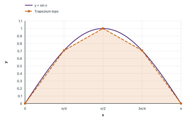
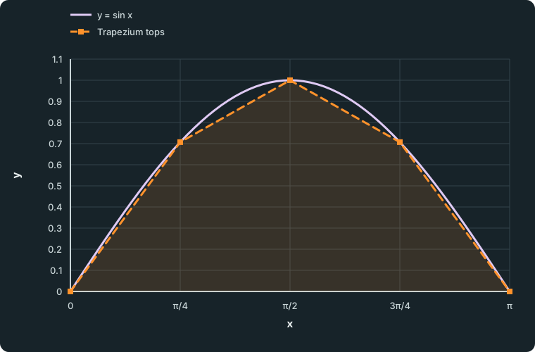
Figure data
This table is included in print while it is open.
| Series | x | y |
|---|---|---|
| y = sin x | 0.000000 | 0.000000 |
| y = sin x | 0.049087 | 0.049067 |
| y = sin x | 0.098175 | 0.098017 |
| y = sin x | 0.147262 | 0.146730 |
| y = sin x | 0.196350 | 0.195091 |
| y = sin x | 0.245437 | 0.242980 |
| y = sin x | 0.294524 | 0.290284 |
| y = sin x | 0.343612 | 0.336890 |
| y = sin x | 0.392699 | 0.382683 |
| y = sin x | 0.441786 | 0.427555 |
| y = sin x | 0.490874 | 0.471397 |
| y = sin x | 0.539961 | 0.514103 |
| y = sin x | 0.589049 | 0.555571 |
| y = sin x | 0.638136 | 0.595699 |
| y = sin x | 0.687223 | 0.634393 |
| y = sin x | 0.736311 | 0.671559 |
| y = sin x | 0.785398 | 0.707107 |
| y = sin x | 0.834486 | 0.740951 |
| y = sin x | 0.883573 | 0.773010 |
| y = sin x | 0.932660 | 0.803207 |
| y = sin x | 0.981748 | 0.831470 |
| y = sin x | 1.030835 | 0.857729 |
| y = sin x | 1.079922 | 0.881921 |
| y = sin x | 1.129010 | 0.903989 |
| y = sin x | 1.178097 | 0.923879 |
| y = sin x | 1.227185 | 0.941544 |
| y = sin x | 1.276272 | 0.956940 |
| y = sin x | 1.325359 | 0.970031 |
| y = sin x | 1.374447 | 0.980785 |
| y = sin x | 1.423534 | 0.989176 |
| y = sin x | 1.472622 | 0.995185 |
| y = sin x | 1.521709 | 0.998795 |
| y = sin x | 1.570796 | 1.000000 |
| y = sin x | 1.619884 | 0.998795 |
| y = sin x | 1.668971 | 0.995185 |
| y = sin x | 1.718058 | 0.989177 |
| y = sin x | 1.767146 | 0.980785 |
| y = sin x | 1.816233 | 0.970031 |
| y = sin x | 1.865321 | 0.956940 |
| y = sin x | 1.914408 | 0.941544 |
| y = sin x | 1.963495 | 0.923880 |
| y = sin x | 2.012583 | 0.903989 |
| y = sin x | 2.061670 | 0.881921 |
| y = sin x | 2.110758 | 0.857728 |
| y = sin x | 2.159845 | 0.831470 |
| y = sin x | 2.208932 | 0.803208 |
| y = sin x | 2.258020 | 0.773010 |
| y = sin x | 2.307107 | 0.740951 |
| y = sin x | 2.356194 | 0.707107 |
| y = sin x | 2.405282 | 0.671559 |
| y = sin x | 2.454369 | 0.634393 |
| y = sin x | 2.503457 | 0.595699 |
| y = sin x | 2.552544 | 0.555570 |
| y = sin x | 2.601631 | 0.514103 |
| y = sin x | 2.650719 | 0.471397 |
| y = sin x | 2.699806 | 0.427555 |
| y = sin x | 2.748894 | 0.382683 |
| y = sin x | 2.797981 | 0.336890 |
| y = sin x | 2.847068 | 0.290285 |
| y = sin x | 2.896156 | 0.242980 |
| y = sin x | 2.945243 | 0.195090 |
| y = sin x | 2.994330 | 0.146731 |
| y = sin x | 3.043418 | 0.098017 |
| y = sin x | 3.092505 | 0.049068 |
| y = sin x | 3.141593 | 0.000000 |
| Trapezium tops | 0.000000 | 0.000000 |
| Trapezium tops | 0.785398 | 0.707107 |
| Trapezium tops | 1.570796 | 1.000000 |
| Trapezium tops | 2.356194 | 0.707107 |
| Trapezium tops | 3.141593 | 0.000000 |
The figure shows why the error has a predictable sign. Where a curve bends downwards (it is concave, f''(x) < 0), each chord lies below the curve, so the trapezium rule underestimates. Where it bends upwards (f''(x) > 0), each chord lies above the curve and the rule overestimates. For sin x on [0,π] with four strips,
which is below the exact value 2. If f'' changes sign inside the interval, the two kinds of error partly cancel and you cannot predict the sign from a sketch alone.
Check your understanding 1
Four strips under a logarithm
Check your understanding 1
Four strips under a logarithm
Use the trapezium rule with 4 strips to estimate ∫₁² ln x dx, giving your answer to 4 decimal places. Then decide whether it is an overestimate or an underestimate without using the exact value.
Show answerHide answer
With h = 0.25 the ordinates are 0, 0.223144, 0.405465, 0.559616, 0.693147. Then
so the estimate is 0.3837 to 4 decimal places. Since d²/(dx²) ln x = -1/x² < 0, the curve bends downwards throughout and every chord lies below it: T₄ is an underestimate. The exact value 2 ln 2-1 ≈ 0.386294 confirms this.
Simpson’s rule fits parabolas
Simpson’s rule takes the strips in pairs. Through the three ordinates of a pair it fits a parabola, and the area under a parabola through (-h,y₀), (0,y₁) and (h,y₂) is exactly
(Write the parabola as px² + qx + c: then y₁ = c and y₀ + y₂ = 2ph² + 2c, while its integral from -h to h is (2/3)ph³ + 2ch. Eliminating p and c gives the expression above.) Adding the pairs gives the rule, which needs an even number of strips:
Along the row of ordinates the weights run 1,4,2,4,2,…,4,1: odd-numbered ordinates are pair midpoints (weight 4), even-numbered interior ordinates are shared by two pairs (weight 2). Because a parabola can follow the bending of a curve, Simpson’s rule is usually far more accurate than the trapezium rule for the same ordinates; it is exact for every cubic.
Worked example 1
Two estimates of π/4
Worked example 1
Two estimates of π/4
Estimate ∫₀¹1/(1 + x²) dx with 4 strips by the trapezium rule and by Simpson’s rule. Compare each estimate with the exact value π/4.
Show full solutionHide solution
Tabulate the ordinates once
Method
Use h = (1-0)/4 = 0.25 and evaluate f(x) = 1/(1 + x²) at the five points.Reason
Both rules use the same five ordinates; only the weights differ. Keep six decimal places so that rounding does not hide the difference between the rules.Working
Answer
r 0 1 2 3 4 xᵣ 0 0.25 0.5 0.75 1 yᵣ 1 0.941176 0.8 0.64 0.5 Apply the trapezium weights 1, 2, 2, 2, 1
Reason
The three interior ordinates each belong to two strips, so they are doubled.Working
Answer
T₄ = 0.25/2[1 + 2(0.941176 + 0.8 + 0.64) + 0.5]; = 0.125 × 6.262353; ≈ 0.782794.Apply the Simpson weights 1, 4, 2, 4, 1
Method
Weight y₁ and y₃ by 4 and y₂ by 2.Reason
y₁ and y₃ are the midpoints of the two pairs of strips; y₂ is the shared end of both pairs.Working
Answer
S₄ = 0.25/3[1 + 4(0.941176 + 0.64) + 2(0.8) + 0.5]; = 9.424706/12; ≈ 0.785392.Compare with the exact value
Working
Answer
π/4 ≈ 0.785398, so the trapezium error is about 0.0026 and the Simpson error about 0.000006: roughly four hundred times smaller from the same five function values.
Quick check
The trapezium estimate is low, but this curve is not concave throughout: f''(x) = (6x²-2)/((1 + x²)³) is negative for x < 1/(square root of 3) and positive after. The underestimates on the left outweigh the overestimates on the right, which you could not have read off a rough sketch.
With the aid of a computer: refine until the digits settle
In 9649 these rules are used “with the aid of a computer”: a spreadsheet or graphing calculator evaluates the ordinates and sums. Your job is to choose n, report the values and judge the accuracy. The usual method is to double n until the required digits stop changing. For I = ∫₀¹e^(-x²) dx ≈ 0.7468241:
| Strips n | Trapezium Tₙ | Error in Tₙ | Simpson Sₙ | Error in Sₙ |
|---|---|---|---|---|
| 2 | 0.731370 | 0.015454 | 0.7471804 | 3.6 × 10⁻⁴ |
| 4 | 0.742984 | 0.003840 | 0.7468554 | 3.1 × 10⁻⁵ |
| 8 | 0.745866 | 0.000959 | 0.7468261 | 2.0 × 10⁻⁶ |
| 16 | 0.746585 | 0.000240 | 0.7468243 | 1.2 × 10⁻⁷ |
Each doubling of n halves h. The trapezium error falls by a factor of about 4, and the Simpson error by a factor of about 16. Simpson’s estimates agree to four decimal places (0.7468) from n = 8; the trapezium rule needs n = 32, where T₃₂ ≈ 0.746764, before it rounds to the same value. When you report a numerical integral, state the rule, the number of strips and the evidence that the quoted digits are stable.
Stepping through a differential equation
For dy/(dx) = f(x,y) with y(x₀) = y₀, the gradient at a known point tells you the direction of the solution curve there. Euler’s method moves a short step h along that tangent:
The gradient changes during the step, so Euler’s method drifts away from the true curve. The improved Euler method first predicts the end of the step with an Euler step, then uses the average of the gradients at the start and at that predicted end:
The predictor uₙ₊₁ is only used inside the second gradient; it is not the answer for that step.
Euler steps drift; improved Euler steps stay close
The solid curve y = e^(−x²) falls from 1 at x = 0 to about 0.367879 at x = 1. Euler points: (0, 1), (0.2, 1), (0.4, 0.92), (0.6, 0.7728), (0.8, 0.587328), (1, 0.399383). Improved Euler points: (0, 1), (0.2, 0.96), (0.4, 0.850944), (0.6, 0.697093), (0.8, 0.528676), (1, 0.372188). At x = 1 the Euler error is about 0.0315 and the improved Euler error about 0.0043.
Scroll across to read every label.
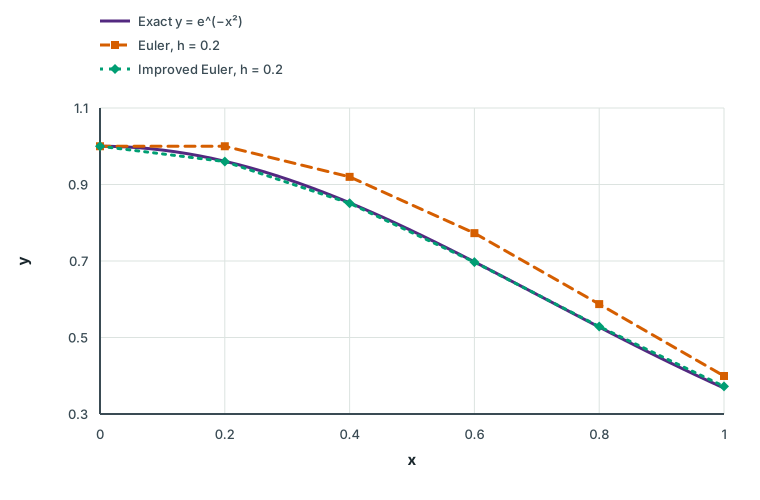
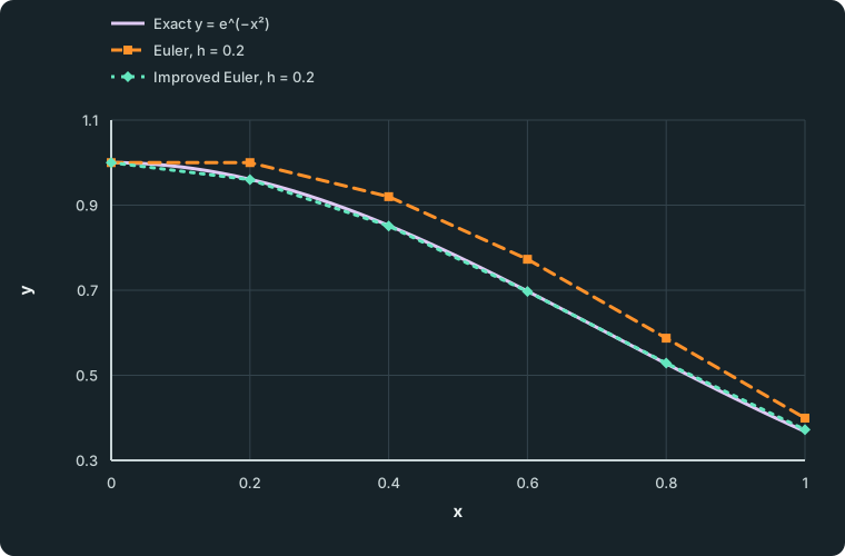
Figure data
This table is included in print while it is open.
| Series | x | y |
|---|---|---|
| Exact y = e^(−x²) | 0.00 | 1.000000 |
| Exact y = e^(−x²) | 0.02 | 0.999600 |
| Exact y = e^(−x²) | 0.04 | 0.998401 |
| Exact y = e^(−x²) | 0.06 | 0.996406 |
| Exact y = e^(−x²) | 0.08 | 0.993620 |
| Exact y = e^(−x²) | 0.10 | 0.990050 |
| Exact y = e^(−x²) | 0.12 | 0.985703 |
| Exact y = e^(−x²) | 0.14 | 0.980591 |
| Exact y = e^(−x²) | 0.16 | 0.974725 |
| Exact y = e^(−x²) | 0.18 | 0.968119 |
| Exact y = e^(−x²) | 0.20 | 0.960789 |
| Exact y = e^(−x²) | 0.22 | 0.952753 |
| Exact y = e^(−x²) | 0.24 | 0.944027 |
| Exact y = e^(−x²) | 0.26 | 0.934634 |
| Exact y = e^(−x²) | 0.28 | 0.924595 |
| Exact y = e^(−x²) | 0.30 | 0.913931 |
| Exact y = e^(−x²) | 0.32 | 0.902668 |
| Exact y = e^(−x²) | 0.34 | 0.890831 |
| Exact y = e^(−x²) | 0.36 | 0.878447 |
| Exact y = e^(−x²) | 0.38 | 0.865541 |
| Exact y = e^(−x²) | 0.40 | 0.852144 |
| Exact y = e^(−x²) | 0.42 | 0.838283 |
| Exact y = e^(−x²) | 0.44 | 0.823987 |
| Exact y = e^(−x²) | 0.46 | 0.809288 |
| Exact y = e^(−x²) | 0.48 | 0.794216 |
| Exact y = e^(−x²) | 0.50 | 0.778801 |
| Exact y = e^(−x²) | 0.52 | 0.763074 |
| Exact y = e^(−x²) | 0.54 | 0.747067 |
| Exact y = e^(−x²) | 0.56 | 0.730811 |
| Exact y = e^(−x²) | 0.58 | 0.714337 |
| Exact y = e^(−x²) | 0.60 | 0.697676 |
| Exact y = e^(−x²) | 0.62 | 0.680859 |
| Exact y = e^(−x²) | 0.64 | 0.663916 |
| Exact y = e^(−x²) | 0.66 | 0.646876 |
| Exact y = e^(−x²) | 0.68 | 0.629770 |
| Exact y = e^(−x²) | 0.70 | 0.612626 |
| Exact y = e^(−x²) | 0.72 | 0.595473 |
| Exact y = e^(−x²) | 0.74 | 0.578336 |
| Exact y = e^(−x²) | 0.76 | 0.561244 |
| Exact y = e^(−x²) | 0.78 | 0.544221 |
| Exact y = e^(−x²) | 0.80 | 0.527292 |
| Exact y = e^(−x²) | 0.82 | 0.510482 |
| Exact y = e^(−x²) | 0.84 | 0.493812 |
| Exact y = e^(−x²) | 0.86 | 0.477305 |
| Exact y = e^(−x²) | 0.88 | 0.460980 |
| Exact y = e^(−x²) | 0.90 | 0.444858 |
| Exact y = e^(−x²) | 0.92 | 0.428956 |
| Exact y = e^(−x²) | 0.94 | 0.413292 |
| Exact y = e^(−x²) | 0.96 | 0.397882 |
| Exact y = e^(−x²) | 0.98 | 0.382740 |
| Exact y = e^(−x²) | 1.00 | 0.367879 |
| Euler, h = 0.2 | 0.00 | 1.000000 |
| Euler, h = 0.2 | 0.20 | 1.000000 |
| Euler, h = 0.2 | 0.40 | 0.920000 |
| Euler, h = 0.2 | 0.60 | 0.772800 |
| Euler, h = 0.2 | 0.80 | 0.587328 |
| Euler, h = 0.2 | 1.00 | 0.399383 |
| Improved Euler, h = 0.2 | 0.00 | 1.000000 |
| Improved Euler, h = 0.2 | 0.20 | 0.960000 |
| Improved Euler, h = 0.2 | 0.40 | 0.850944 |
| Improved Euler, h = 0.2 | 0.60 | 0.697093 |
| Improved Euler, h = 0.2 | 0.80 | 0.528676 |
| Improved Euler, h = 0.2 | 1.00 | 0.372188 |
Worked example 2
One curve, two methods
Worked example 2
One curve, two methods
For dy/(dx) = -2xy with y(0) = 1, use a step h = 0.2 to estimate y(0.4) by Euler’s method and by the improved Euler method. Compare both with the exact solution y = e^(-x²).
Show full solutionHide solution
Euler: follow the starting gradient each step
Reason
Each step uses only the gradient at its left-hand point.Working
Answer
y₁ = 1 + 0.2 × (-2 × 0 × 1) = 1,; y₂ = 1 + 0.2 × (-2 × 0.2 × 1) = 0.92.Improved Euler, first step
Method
Predict, then average the start and predicted-end gradients.Reason
The gradient changes during the step; the average of its two end values follows the curve more closely than either alone.Working
Answer
f(0,1) = 0, u₁ = 1 + 0.2 × 0 = 1,; f(0.2,u₁) = -2(0.2)(1) = -0.4,; y₁ = 1 + 0.1 (0-0.4) = 0.96.Improved Euler, second step
Method
Start from the corrected value y₁ = 0.96, not from the predictor.Reason
The predictor was only a tool for finding the end gradient of the first step.Working
Answer
f(0.2,0.96) = -0.384, u₂ = 0.96 + 0.2(-0.384) = 0.8832,; f(0.4,0.8832) = -2(0.4)(0.8832) = -0.70656,; y₂ = 0.96 + 0.1 (-0.384-0.70656) = 0.850944.Compare with the exact value
Working
Answer
y(0.4) = e^(-0.16) ≈ 0.852144. Euler’s estimate 0.92 is about 0.068 too large; the improved estimate 0.850944 is about 0.0012 too small.
Quick check
The curve is falling more and more steeply here, so the gradient at the start of each step is too gentle and Euler’s method stays above the curve. Averaging in the steeper end gradient corrects most of that error. Halving h roughly halves Euler’s error but quarters the improved method’s.
Spot the mistake 1
Which y belongs in the second gradient?
Spot the mistake 1
Which y belongs in the second gradient?
Continuing the same problem from (0.2, 0.96), a student writes the next improved Euler step as
Find the error and correct the step.
Write your answer, then compare it with the solution
Show full solutionHide solution
Locate the wrong input
Method
The end gradient was evaluated at the old height y = 0.96.Reason
The end gradient must be taken where the solution is predicted to be at x = 0.4. The curve has moved down during the step, so the old height belongs to a different point.Working
Answer
Predict first: u₂ = 0.96 + 0.2(-0.384) = 0.8832. Then
y₂ = 0.96 + 0.1[-0.384 + f(0.4,0.8832)]; = 0.96 + 0.1 (-0.384-0.70656); = 0.850944.
Common mistake
Using f(xₙ₊₁,yₙ) is tempting because yₙ is the only height already known. But the formula needs the gradient at the end of the step, and that requires an estimate of the end height. Here the mistake gives 0.8448, an error of 0.0073, six times the correct method’s error.
Check your understanding 2
Two methods, two steps
Check your understanding 2
Two methods, two steps
For dy/(dx) = x + y with y(0) = 1, use h = 0.1 to estimate y(0.2) by Euler’s method and by the improved Euler method. The exact solution is y = 2e^x-x-1.
Show answerHide answer
Euler’s method:
Improved Euler method:
The exact value is 2e^(0.2)-1.2 ≈ 1.242806. Euler’s error is about 0.023 and the improved method’s about 0.0008. Both estimates are low because the solution curve bends upwards, so each starting gradient is too gentle.
Common mistakes
- Using n ordinates instead of n + 1, so that h is wrong.
- Giving every ordinate weight 2 in the trapezium rule, or forgetting to double the interior ones.
- Using Simpson’s rule with an odd number of strips, or swapping the weights 4 and 2.
- Predicting over- or underestimation from whether a curve is rising, instead of from the sign of f''(x).
- In the improved Euler method, evaluating the end gradient at the old height, or carrying the predictor forward as the next value.
- Rounding ordinates or intermediate values early. Keep at least two more digits than the answer requires.
Before you move on
Try it yourself 1
Distance from a speed log
Try it yourself 1
Distance from a speed log
A car’s speed v in m s⁻¹ is logged every 2 seconds:
| t (s) | 0 | 2 | 4 | 6 | 8 |
|---|---|---|---|---|---|
| v (m s⁻¹) | 0 | 5.2 | 9.1 | 11.8 | 13.0 |
Estimate the distance travelled in the 8 seconds by the trapezium rule and by Simpson’s rule. Then decide, from the data alone, whether the trapezium estimate is likely to be too small or too large.
Try this before viewing the solution
Show full solutionHide solution
Distance is the area under the speed–time graph
Method
With h = 2, apply both rules to the five recorded speeds.Reason
There is no formula for v; the rules only need the tabulated values.Working
Answer
T = 2/2[0 + 2(5.2 + 9.1 + 11.8) + 13.0] = 65.2 m,; S = 2/3[0 + 4(5.2 + 11.8) + 2(9.1) + 13.0] = (2/3)(99.2) ≈ 66.1 m.Judge the direction of the error
Working
Answer
The speed rises by 5.2, 3.9, 2.7 and 1.2 m s⁻¹ in successive intervals, so the graph bends downwards. Straight chords lie below such a curve, so the trapezium estimate 65.2 m is likely to be too small. Simpson’s estimate, about 66.1 m, follows the bending and is the better estimate.
Quick check
The two estimates differ by under 1 m, about 1.4%. With readings every 2 s you cannot refine h, so the honest statement is “about 66 m”, with Simpson’s value preferred.
Loading reading progress…
Lesson done
- Monday
- Tuesday
- Wednesday
- Thursday
- Friday
- Saturday
- Sunday
Checking learning on this device…
Change goal
Progress options
Loading questions…