Separation, initial values and lost solutions
Retain equilibrium solutions, transform derivatives and initial-value domains, and formulate rate models with physical limits.
More
Offline pages
Saved on this device only. Connect at least once every 30 days to confirm Premium. Sign-out or a change of account removes saved copies.
Find this activity in your course
On this page
You stopped at:
ContinueRevision Mode is on. Questions and activities are hidden.
A rate rule describes a family of curves
Knowing a quantity’s initial value does not describe how it changes. A differential equation supplies a rule for its derivative; an initial condition selects a curve from the possible solutions. A solution must satisfy the equation at every point of its stated interval, as well as passing through the initial point.
For example, consider
Before dividing by y, test y = 0 in the original equation. Its derivative is zero and the right-hand side is also zero, so it is a constant, or equilibrium, solution.
On an interval where y ≠ 0, separate the variables and integrate:
The absolute value permits both signs of y. Exponentiating gives y = Ae^(x²/2) with a nonzero real A at this stage. Restore the equilibrium by allowing A = 0 too. The complete family is
Differentiation gives y' = Axe^(x²/2) = xy, including when A is zero or negative. If y(0) = 2, then A = 2, giving a particular solution valid for all real x.
Check a divisor before separating
For an equation of the form dy/dx = f(x)g(y), first check the values where g(y) = 0. Each allowed constant value satisfying the original equation is an equilibrium solution. Dividing by g(y) excludes those values from that separation step.
On an interval where the divisor is nonzero, write
This reverses a chain rule: if H'(y) = 1/g(y), then dH(y(x))/dx = y'/g(y) = f(x). The dependent quantity y changes with x; integrating f(x)g(y) while treating y as a constant would not solve the original rate equation.
Check your understanding 1 Restore the solution lost by division
Solve dy/dx = 2y, including its equilibrium solution, and apply y(0) = -3. Explain how using ln y instead of ln |y| would affect this initial-value problem. Check the final function by differentiation.
Show answer
The equilibrium is y = 0. For nonzero y, separation gives ln |y| = 2x + C, hence y = Ae^2x. Allowing any real A restores zero and retains negative solutions. The initial condition gives A = -3, so y = -3e^2x for every real x.
Its derivative is -6e^2x = 2y, and its value at zero is -3. A real ln y requires y > 0 and would wrongly exclude the required negative branch.
A separated family and the equilibrium solutions may be written together or separately. What matters is checking every restriction introduced during the derivation. A lost equilibrium is not recovered by assigning an invalid value to an integration constant.
An initial condition selects an interval as well as a constant
For dy/dx = x(1 + y²), separation gives
With y(0) = 0, the local solution is y = tan(x²/2). Its derivative is x sec² (x²/2) = x(1 + y²) wherever the function is finite. Here angles are in radians.
The first poles on either side of the initial point occur at x = ± square root of π, where the tangent’s input is π/2. Thus the maximal connected interval containing the initial point is
The formula can be evaluated on other intervals between poles, but those pieces do not form one finite, continuous initial-value solution through zero. Check a denominator, logarithm, inverse-function branch or pole before extending a solution’s interval.
Check your understanding 2 Keep the interval containing the initial point
Solve dy/dx = (y-1)² with y(0) = 2. State the maximal interval containing zero, identify the equilibrium excluded by division, and verify the particular solution in the original equation.
Show answer
The equilibrium is y = 1. For y ≠ 1, integration gives -1/(y-1) = x + C, hence y = 1-1/(x + C). The initial condition gives C = -1, so y = 1 + 1/(1-x).
Its derivative is 1/(1-x)² = (y-1)², and y(0) = 2. The pole at x = 1 separates its intervals. The maximal interval containing zero is x < 1; values on x > 1 do not extend this initial-value solution across the pole. The separate equilibrium does not satisfy the stated initial value.
A substitution changes the derivative too
Some equations become separable after a given change of variable. For
use the given substitution u = x + y. Since u depends on both terms,
The additional one is essential: the new derivative is not simply dy/dx. Check the transformed equation’s equilibrium first. The solution u = 0 gives y = -x, whose derivative -1 agrees with (x + y)²-1 = -1. An equilibrium in the new variable can correspond to a nonconstant original function.
For u ≠ 0, separate and integrate:
Returning to y gives y = -x-1/(x + C), with x + C ≠ 0, alongside the separate solution y = -x. For y(0) = 1, we obtain C = -1 and
Differentiate the final expression: y' = 1/(1-x)²-1. Since x + y = 1/(1-x), substitution into the original right-hand side gives the same result. The separate solution y = -x does not satisfy y(0) = 1.
Check your understanding 3 Differentiate the full change of variable
For x > 0, an equation is dy/dx = y/x + (y/x)². Use the given substitution u = y/x to solve it, retaining any solution excluded by division. Then apply y(1) = 1 and state the maximal interval through that initial point. Explain which restriction comes from the original equation and which comes from the solution.
Show answer
Write y = xu, so y' = u + xu'. Substitution gives u + xu' = u + u², or xu' = u². The equilibrium u = 0 yields y = 0. For nonzero u, -1/u = ln x + C, so y = -x/(ln x + C) on suitable intervals with x > 0 and ln x + C ≠ 0.
The initial condition gives C = -1, hence y = x/(1- ln x). Its derivative is (2- ln x)/(1- ln x)², agreeing with y/x + (y/x)². The original equation restricts x > 0; the particular solution has a pole at x = e. The maximal interval containing x = 1 is 0 < x < e. The separate zero solution does not meet this initial condition.
Form a model from the quantity that controls the rate
Suppose an ideal temperature model says that the rate of change of an object’s temperature T is proportional to its difference from a fixed ambient temperature Tₐ. Let t be measured in minutes. To model movement towards that ambient value, use
The coefficient k has units min⁻¹. When T > Tₐ, the rate is negative; when T < Tₐ, it is positive. The same equation permits cooling or warming. This assumes a constant ambient temperature, one representative object temperature and a constant rate coefficient over the modelled period.
Put U = T-Tₐ. Since Tₐ is constant, U' = -kU. The exponential family and its equilibrium give
where T₀ is the initial temperature. The signed initial excess T₀-Tₐ must be retained. If it is zero, the temperature stays at Tₐ. Otherwise its sign stays fixed because e^(-kt) > 0: the model approaches the ambient value without crossing it or reaching it at a finite time.
For Tₐ = 20 °C, T₀ = 80 °C and T(10) = 50 °C,
so k = (ln 2)/10 min⁻¹. The initial excess halves every ten minutes under this model. In particular, T(20) = 20 + 60/4 = 35 °C.
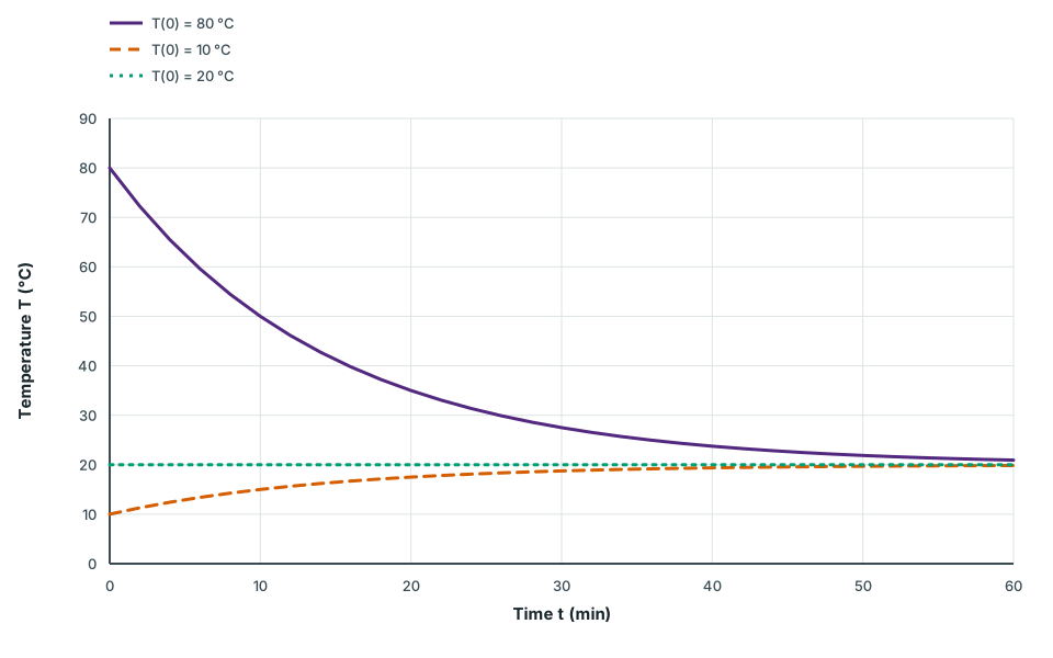
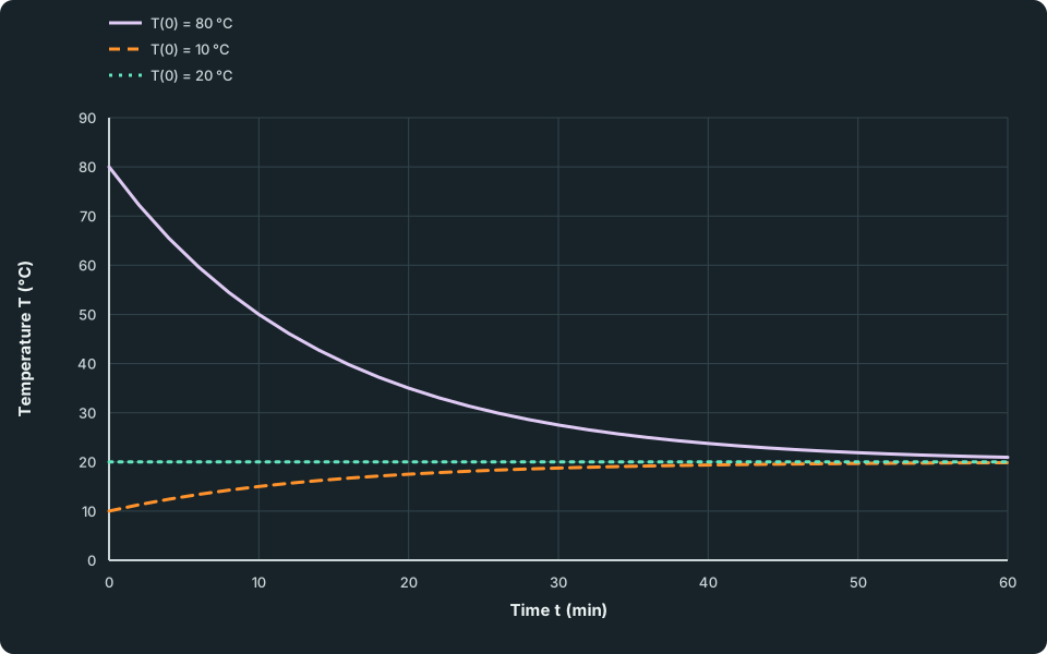
One rate law with three initial temperatures
The 80 °C solution decreases to 50 °C after 10 minutes and 35 °C after 20 minutes, approaching 20 °C from above. The 10 °C solution increases to 15 °C after 10 minutes and approaches 20 °C from below. The equilibrium remains constant. Neither changing curve crosses the equilibrium under this model.
Scroll across the figure to read all labels.
View figure data
| Time t (min) | T(0) = 80 °C | T(0) = 10 °C | T(0) = 20 °C |
|---|---|---|---|
| 0 | 80.00 | 10.00 | 20 |
| 2 | 72.23 | 11.29 | 20 |
| 4 | 65.47 | 12.42 | 20 |
| 6 | 59.59 | 13.40 | 20 |
| 8 | 54.46 | 14.26 | 20 |
| 10 | 50.00 | 15.00 | 20 |
| 12 | 46.12 | 15.65 | 20 |
| 14 | 42.74 | 16.21 | 20 |
| 16 | 39.79 | 16.70 | 20 |
| 18 | 37.23 | 17.13 | 20 |
| 20 | 35.00 | 17.50 | 20 |
| 22 | 33.06 | 17.82 | 20 |
| 24 | 31.37 | 18.11 | 20 |
| 26 | 29.90 | 18.35 | 20 |
| 28 | 28.62 | 18.56 | 20 |
| 30 | 27.50 | 18.75 | 20 |
| 32 | 26.53 | 18.91 | 20 |
| 34 | 25.68 | 19.05 | 20 |
| 36 | 24.95 | 19.18 | 20 |
| 38 | 24.31 | 19.28 | 20 |
| 40 | 23.75 | 19.38 | 20 |
| 42 | 23.26 | 19.46 | 20 |
| 44 | 22.84 | 19.53 | 20 |
| 46 | 22.47 | 19.59 | 20 |
| 48 | 22.15 | 19.64 | 20 |
| 50 | 21.88 | 19.69 | 20 |
| 52 | 21.63 | 19.73 | 20 |
| 54 | 21.42 | 19.76 | 20 |
| 56 | 21.24 | 19.79 | 20 |
| 58 | 21.08 | 19.82 | 20 |
| 60 | 20.94 | 19.84 | 20 |
The three curves use the same coefficient and ambient temperature with different initial values. They show why the equilibrium must survive division by T-20 and why a negative initial excess must remain available in the solution family.
Check your understanding 4 Interpret the difference from the reference value
For the calibrated model starting at 80 °C, find the first time the temperature is at most 25 °C. Give an exact time and an approximation to two decimal places. Does this model predict a time when the temperature becomes exactly 20 °C? State which assumptions would need reconsideration if the ambient temperature changed during the observation.
Show answer
The threshold is 60e^(-kt) ≤ 5, giving t ≥ ln 12/k = 10 ln 12/ln 2 minutes. The first time is approximately 35.85 minutes. There is no finite time at which the positive exponential excess becomes zero; 20 °C is the limiting temperature.
The equation and solution assume a constant Tₐ. A changing ambient temperature changes that model, and the fitted constant-coefficient solution cannot be used without reconsidering the assumptions. A long-term mathematical limit is a prediction under those assumptions, not a guarantee about every physical observation.
Try it yourself 1
Track the amount in a filling tank
Problem
A tank initially contains 100 litres of well-mixed liquid with 10 grams of dissolved salt. Pure water enters at 4 litres per minute, and well-mixed liquid leaves at 2 litres per minute. Assume constant flow rates and no other volume or salt changes while the tank fills. Its capacity is 180 litres; study only the period up to that capacity, with no overflow.
Let S(t) be the salt amount in grams after t minutes. The outgoing salt concentration is the current amount divided by the current liquid volume. Form and solve a differential equation for S. Find the salt amount and concentration at t = 25, and decide whether the concentration can fall to 0.025 g/L before the tank fills. A proposed model is S' = -2S/100: explain which stated condition it loses. Check the solution and its valid time interval.
Write your answer, then compare it with the solution
Hints
Hint 1
Separate amount, concentration and flow rate
Find the net volume change before writing the salt balance. Convert the outgoing volume rate into a salt rate using the concentration at that same time. Keep the capacity condition when interpreting a predicted threshold time.
Show full solution
Track the changing volume and salt balance
Method
Use net flow for volume and amount-in minus amount-out for salt.Reason
The two volume rates differ, while incoming pure water supplies no salt.Working
Answer
The volume is V(t) = 100 + 2t litres and reaches 180 litres at t = 40. The outgoing concentration is S/(100 + 2t) g/L, so S' = -2S/(100 + 2t) = -S/(50 + t) g/min while the flows continue. The proposed fixed denominator 100 ignores the increasing volume. Its salt-loss rate is correct only at the initial instant.Separate and apply the initial amount
Method
Solve the rate equation on the modelled time interval.Reason
The time-dependent dilution factor remains a known function of t, so the equation is separable.Working
Answer
For positive S, dS/S = -dt/(50 + t), giving S = K/(50 + t). Since S(0) = 10, K = 500 and S(t) = 500/(50 + t). Its derivative is -500/(50 + t)² = -S/(50 + t), and it has the required initial value. The zero-amount equilibrium also solves the rate equation, but does not meet this initial condition. The amount formula applies throughout 0 ≤ t ≤ 40, with the flow-rate equation describing the period before capacity is reached.Find amount and concentration at the requested time
Method
Use the amount and volume at the same instant.Reason
Grams of salt and grams per litre answer different questions.Working
Answer
At t = 25, the volume is 150 litres and S = 500/75 = 20/3 grams. The concentration is (20/3)/150 = 2/45 g/L. More generally it is S/V = 250/(50 + t)² g/L. Both amount and concentration decrease, with no salt entering.Check the threshold against capacity
Method
Solve the concentration condition, then apply the physical time boundary.Reason
An algebraic prediction outside the modelled interval does not establish an outcome before the tank fills.Working
Answer
The equation 250/(50 + t)² = 0.025 gives 50 + t = 100 for t ≥ 0, hence t = 50. This lies beyond t = 40, so the threshold is not reached before capacity. At capacity the concentration is 250/90² = 5/162 g/L, still greater than 0.025 g/L. Continuing the same formula beyond capacity would require different physical assumptions.
Quick check
Compare volume, salt amount and concentration separately, with units on each rate. A constant-volume exponential model uses different assumptions from this filling tank. The initial condition, original equation and capacity boundary all belong in the final check.
Before separating, test excluded values in the original equation. After integrating or changing variables, return to the original quantity, apply the initial condition and select its connected solution interval. For a contextual prediction, also check the rate’s sign, units and the period during which the model’s assumptions hold.
Keep track of this lesson
Mark the lesson done when you have worked through it.
Lesson progress is optional and kept on this device.
Loading lesson controls…
Your lesson mark records your own study. Checks are kept separately in My Learning.