Correlation, regression and prediction
Interpret scatter and residuals, fit each prediction direction, and assess range, outliers and causal claims.
Practise
More
Offline pages
Saved on this device only. Connect at least once every 30 days to confirm Premium. Sign-out or a change of account removes saved copies.
Find this activity in your course
On this page
You stopped at:
ContinueRevision Mode is on. Questions and activities are hidden.
Inspect the scatter before summarising it
A scatter diagram places one point for each paired observation (x,y). Keep each x with the y measured on the same case. Sorting the columns separately would invent different pairings and a different relationship.
Look for the direction, whether a straight line is plausible, unusual observations and the range actually represented. Product-moment correlation r summarises the strength and direction of a linear association, with -1 ≤ r ≤ 1 when it is defined:
- r near 1 indicates strong positive linear association;
- r near −1 indicates strong negative linear association;
- r near zero indicates little linear association, but can accompany a strong curved pattern.
The magnitude describes linear strength; the sign describes direction. A value −0.98 is not a weaker linear fit merely because it is numerically less than 0.6. Also, r has no units: changing metres to centimetres in a column does not change r. It is not a percentage of correctly predicted cases.
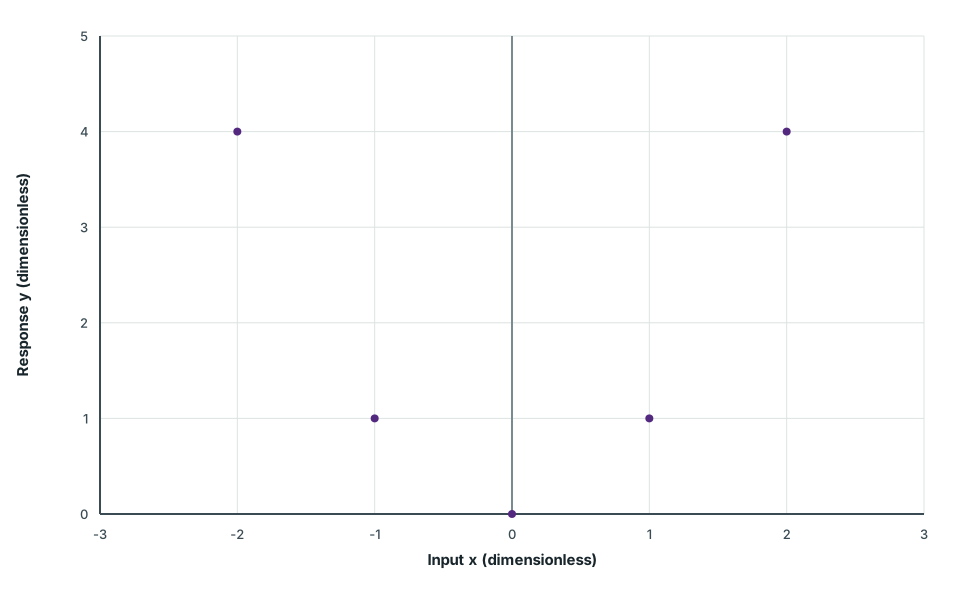
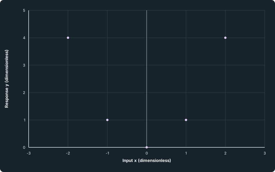
Zero linear correlation can accompany a curved pattern
Points fall from y = 4 at x = −2 to y = 0 at x = 0 and rise symmetrically to y = 4 at x = 2. The pattern is curved rather than a rising or falling straight-line trend.
Scroll across the figure to read all labels.
View figure data
| Input x (dimensionless) | Observed pairs |
|---|---|
| -2 | 4 |
| -1 | 1 |
| 0 | 0 |
| 1 | 1 |
| 2 | 4 |
In this five-point example r = 0, yet the points fall and rise in a clear pattern. “No linear association” and “no relationship” are different claims. If either data column is constant, its correlation with the other column is undefined; do not replace a missing correlation by zero.
Check your understanding 1 Read direction and strength separately
One scatter has r = −0.98, another has r = 0.6, and the U-shaped scatter above has r = 0. Which of the first two has stronger linear association? What can you conclude from the third value? What happens to the first correlation if all x measurements are converted from metres to centimetres, or if every x value were the same?
Show answer
The first has stronger linear association because 0.98 exceeds 0.6 in magnitude, with a negative rather than positive direction. The third has zero linear correlation, but the curved scatter shows that this is not absence of a relationship.
Converting metres to centimetres multiplies every x by the same positive constant and leaves r = −0.98. If all x values were identical, there would be no x variation for the correlation calculation, so r would be undefined, not zero. These are different data conditions.
A regression line has a prediction direction
The least-squares regression of y on x predicts y from a given x. It chooses its intercept and gradient to minimise the sum of squared vertical residuals. If the predicted value is ŷ, the residual is observed minus predicted:
A positive residual places the observation above the fitted line; a negative residual places it below. Squaring stops positive and negative errors cancelling in the quantity being minimised.
For the paired data (1,2), (2,4), (3,5) and (4,7), enter the matching x and y lists into a calculator or graphing tool and select a linear y-on-x fit with an intercept. The result is
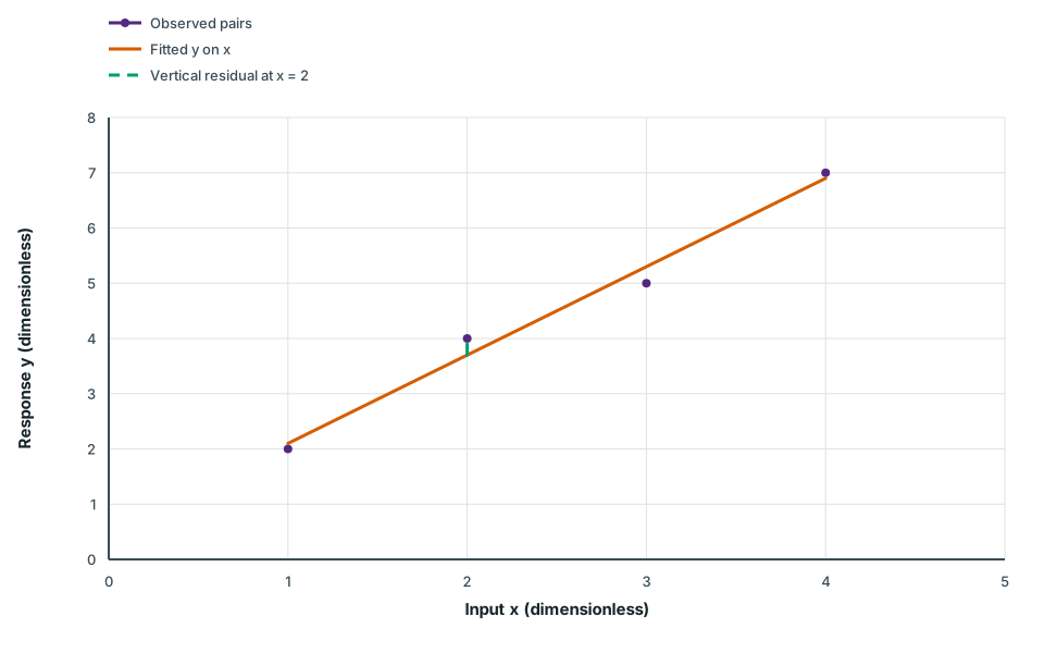
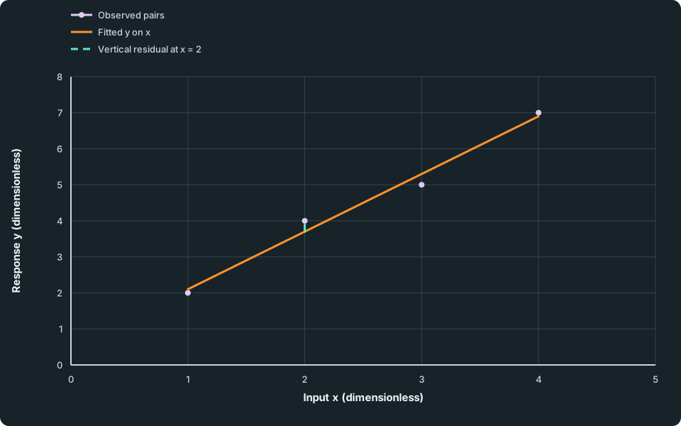
At x = 2, the prediction is 3.7 while the observation is 4, so the vertical residual is 0.3. The line need not pass through every observation. It does pass through the mean pair (2.5,4.5), as a least-squares line with an intercept should.
A fitted line and an observed vertical residual
Circular markers show four paired observations close to a rising straight line. The fitted line runs only from x = 1 to x = 4. A short dashed vertical segment at x = 2 joins the fitted value 3.7 to the observed value 4.
Scroll across the figure to read all labels.
View figure data
| Series | Input x (dimensionless) | Response y (dimensionless) |
|---|---|---|
| Observed pairs | 1.00 | 2.00 |
| Observed pairs | 2.00 | 4.00 |
| Observed pairs | 3.00 | 5.00 |
| Observed pairs | 4.00 | 7.00 |
| Fitted y on x | 1.00 | 2.10 |
| Fitted y on x | 1.05 | 2.18 |
| Fitted y on x | 1.10 | 2.26 |
| Fitted y on x | 1.15 | 2.34 |
| Fitted y on x | 1.20 | 2.42 |
| Fitted y on x | 1.25 | 2.50 |
| Fitted y on x | 1.30 | 2.58 |
| Fitted y on x | 1.35 | 2.66 |
| Fitted y on x | 1.40 | 2.74 |
| Fitted y on x | 1.45 | 2.82 |
| Fitted y on x | 1.50 | 2.90 |
| Fitted y on x | 1.55 | 2.98 |
| Fitted y on x | 1.60 | 3.06 |
| Fitted y on x | 1.65 | 3.14 |
| Fitted y on x | 1.70 | 3.22 |
| Fitted y on x | 1.75 | 3.30 |
| Fitted y on x | 1.80 | 3.38 |
| Fitted y on x | 1.85 | 3.46 |
| Fitted y on x | 1.90 | 3.54 |
| Fitted y on x | 1.95 | 3.62 |
| Fitted y on x | 2.00 | 3.70 |
| Fitted y on x | 2.05 | 3.78 |
| Fitted y on x | 2.10 | 3.86 |
| Fitted y on x | 2.15 | 3.94 |
| Fitted y on x | 2.20 | 4.02 |
| Fitted y on x | 2.25 | 4.10 |
| Fitted y on x | 2.30 | 4.18 |
| Fitted y on x | 2.35 | 4.26 |
| Fitted y on x | 2.40 | 4.34 |
| Fitted y on x | 2.45 | 4.42 |
| Fitted y on x | 2.50 | 4.50 |
| Fitted y on x | 2.55 | 4.58 |
| Fitted y on x | 2.60 | 4.66 |
| Fitted y on x | 2.65 | 4.74 |
| Fitted y on x | 2.70 | 4.82 |
| Fitted y on x | 2.75 | 4.90 |
| Fitted y on x | 2.80 | 4.98 |
| Fitted y on x | 2.85 | 5.06 |
| Fitted y on x | 2.90 | 5.14 |
| Fitted y on x | 2.95 | 5.22 |
| Fitted y on x | 3.00 | 5.30 |
| Fitted y on x | 3.05 | 5.38 |
| Fitted y on x | 3.10 | 5.46 |
| Fitted y on x | 3.15 | 5.54 |
| Fitted y on x | 3.20 | 5.62 |
| Fitted y on x | 3.25 | 5.70 |
| Fitted y on x | 3.30 | 5.78 |
| Fitted y on x | 3.35 | 5.86 |
| Fitted y on x | 3.40 | 5.94 |
| Fitted y on x | 3.45 | 6.02 |
| Fitted y on x | 3.50 | 6.10 |
| Fitted y on x | 3.55 | 6.18 |
| Fitted y on x | 3.60 | 6.26 |
| Fitted y on x | 3.65 | 6.34 |
| Fitted y on x | 3.70 | 6.42 |
| Fitted y on x | 3.75 | 6.50 |
| Fitted y on x | 3.80 | 6.58 |
| Fitted y on x | 3.85 | 6.66 |
| Fitted y on x | 3.90 | 6.74 |
| Fitted y on x | 3.95 | 6.82 |
| Fitted y on x | 4.00 | 6.90 |
| Vertical residual at x = 2 | 2.00 | 3.70 |
| Vertical residual at x = 2 | 2.00 | 4.00 |
Check your understanding 2 Check the fitted line against the observations
For the four paired observations and fitted line above, calculate the residual at each x and the sum of their squares. Explain why simply summing the signed residuals would conceal their spread. A claim says r ≈ 0.992278 means about 99.2% of observations have been predicted exactly; assess it against your results.
Show answer
The predictions at x = 1, 2, 3 and 4 are 2.1, 3.7, 5.3 and 6.9. Subtracting each from the observed y gives residuals −0.1, 0.3, −0.3 and 0.1. Their sum is zero, but their squared sum is 0.01 + 0.09 + 0.09 + 0.01 = 0.2.
The residuals are not all zero, so cancellation does not mean a perfect fit. Correlation measures linear association, not a fraction of exact predictions: none of these four predictions is exactly its observation, despite the high r.
For the x-on-y regression, the input is a given y and the output is a predicted x. Its fitting criterion minimises squared horizontal x residuals instead. For the same four points, that separately fitted line is approximately
Algebraically rearranging the y-on-x line gives x = -0.3125 + 0.625y, which has different coefficients. It describes the same original line viewed backwards, rather than minimising the reverse prediction errors. When choosing between two predictive fits for paired observational data, select the line by the response you need to estimate, not by whichever equation appears first on the calculator.
A different question may supply a calibration model and ask which input makes its fitted output reach a target. Solve that specified model. Inverting it for that purpose does not create a new reverse least-squares fit.
Check your understanding 3 Which variable is being predicted?
A study fits both height-on-age and age-on-height regression lines. Which should be used to estimate height from a given age, and why is algebraically reversing that line not generally the age-on-height fit? State the roles of the input, prediction and residual in each direction.
Show answer
Use height-on-age: age is given and height is predicted, with vertical height residuals minimised when age is plotted horizontally. For age-on-height, height is given and age is predicted; the fit minimises age residuals instead.
Rearranging the first equation does not generally minimise those reverse errors. The two lines are separately fitted for their prediction directions. The relevant age or height range and the population studied still matter for either prediction.
Check your understanding 4 Separate reverse prediction from calibration inversion
For the original paired observations (1,2), (2,4), (3,5), (4,7), use the y-on-x fit to predict y at x = 2. Next, use the separately fitted x-on-y line to predict x at y = 4. Finally, solve the original y-on-x calibration model for the input that gives a fitted output of 4. Give the two x results to four decimal places and explain why they differ.
Show answer
The y-on-x fit is ŷ = 0.5 + 1.6x, so its prediction at x = 2 is 3.7. The independently fitted reverse line is x hat = -7/26 + (8/13)y. At y = 4 it predicts 57/26 ≈ 2.1923.
For the calibration question, keep the specified y-on-x model and solve 4 = 0.5 + 1.6x. This gives x = 35/16 = 2.1875. It finds the input whose fitted output reaches the target; it is not a new least-squares fit for x. The reverse fit minimises x residuals, whereas the original fit minimises y residuals. Changing the question changes which calculation is appropriate, even though both results use the same observed pairs.
Distinguish interpolation from extrapolation
For the original four-point example, x = 2.5 lies within the observed x-range 1 to 4. Its prediction ŷ = 4.5 is an interpolation. At x = 20, the line gives 32.5, but this is an extrapolation far outside that range. A high r inside the observed range does not establish that the relationship continues there.
Interpolation is better supported by the observed range, but it is not a guarantee for an individual. Keep the prediction’s units, the fitted population and the remaining scatter in view. For a reverse prediction from y, check the observed y-range instead of checking only the x-range.
A prediction needs a setting
An unusual point can change both r and the fitted line substantially. Adding (8,0) to the original four points changes r from approximately 0.992278 to −0.404110 and the fitted y-on-x gradient from 1.6 to approximately −0.404110. Inspect such a point: a recording error, a different process and a genuine extreme observation have different implications. Do not delete it merely to obtain a stronger correlation.
Association alone does not establish causation. A third variable or selection process can explain why two quantities move together. Also, a line fitted to one population need not predict another population accurately just because its variables have the same names.
Report what went into a fit: paired variables and units, the chosen regression direction, coefficients with sufficient precision, data range and the limitations relevant to the prediction. Keep unrounded coefficients for calculations, then round the final prediction as requested.
Try it yourself 1
Use a small observational study
Problem
An illustrative study records weekly practice time x in hours and a test score y on a scale from 0 to 10 for five participants:
| x (hours) | y (points) |
|---|---|
| 1 | 2 |
| 2 | 5 |
| 3 | 4 |
| 4 | 8 |
| 5 | 6 |
Use a calculator or graphing tool to fit y on x and x on y, and find r. Use the appropriate fit to predict the score for x = 3.5 and the practice time for a participant with y = 7. Give these predictions to two decimal places. For the observed pair (3,4), find the y residual.
Finally calculate the score predicted at x = 9 and assess it against the data range and score scale. Explain whether the association establishes that making a participant practise for more hours will cause the predicted score increase.
Write your answer, then compare it with the solution
Hints
Hint 1
Identify the given quantity in each prediction
Keep each participant’s time and score together in the calculator lists. For each requested estimate, identify the response to be predicted and use the fit that minimises errors in that response. Check the relevant input range before interpreting it.
Show full solution
Fit both prediction directions to the paired lists
Method
Read the intercept, gradient and correlation with the variable roles stated.Reason
The two least-squares criteria minimise different response errors.Working
Answer
The y-on-x fit is y hat = 1.7 + 1.1x. The x-on-y fit is x hat = 0.25 + 0.55y. The product-moment correlation is approximately 0.777817. Both fits pass through the mean pair (3,5), but rearranging the first gives a different reverse equation.Choose the fitted response for each estimate
Method
Use y on x for a given time and x on y for a given score.Reason
The question changes which variable is known.Working
Answer
At x = 3.5, y hat = 1.7 + 1.1(3.5) = 5.55 points. At y = 7, x hat = 0.25 + 0.55(7) = 4.10 hours. These inputs lie within the respective observed ranges x = 1 to 5 and y = 2 to 8. At (3,4), the y prediction is 5, so the residual is 4 − 5 = −1 point.Assess the model beyond the fitted observations
Method
Calculate the distant prediction, then check whether its interpretation is credible.Reason
A formula can return a number outside the measurement scale, and observational association does not establish an intervention’s effect.Working
Answer
At x = 9, the line predicts 1.7 + 1.1(9) = 11.6 points. This extrapolates beyond the sampled practice range and exceeds the test’s maximum of 10, so it cannot be a valid score prediction on that scale. The small observational study does not establish that extra practice alone causes the fitted change; other differences between participants or their selection may explain the association. Even the interpolated estimates are fitted predictions, not guaranteed individual outcomes.
Quick check
Compare the paired lists, direction of each fit, residual sign, input range and contextual conclusion separately. A coefficient or correlation without the population and measurement meaning is not a complete prediction argument.
Keep track of this lesson
Mark the lesson done when you have worked through it.
Lesson progress is optional and kept on this device.
Loading lesson controls…
Your lesson mark records your own study. Checks are kept separately in My Learning.