Transformed regression and original scales
Fit square, reciprocal and logarithmic models, recover predictions and compare errors on their stated scales.
More
Offline pages
Saved on this device only. Connect at least once every 30 days to confirm Premium. Sign-out or a change of account removes saved copies.
Find this activity in your course
On this page
You stopped at:
ContinueRevision Mode is on. Questions and activities are hidden.
A curved model can be linear in a transformed input
A straight-line fit is a model for the two variables actually entered. If the proposed relationship is y = a + bx², define X = x² and fit y on X. The intercept estimates a and the gradient estimates b. Fitting y on the original x would estimate a different model.
Consider these illustrative paired measurements:
| x (s) | X = x² (s²) | y (cm) |
|---|---|---|
| 1 | 1 | 5 |
| 2 | 4 | 13 |
| 3 | 9 | 30 |
| 4 | 16 | 50 |
The original scatter bends upwards. Entering X = 1, 4, 9, 16 as the input column and the same y values as response gives the fitted line
with r ≈ 0.999243 on these transformed axes. Substituting X = x² recovers the original-scale model
The intercept has unit cm and the coefficient of x² has unit cm/s². For x = 2.5 s, substitute X = 6.25 s² to get approximately 20.7016 cm. Substituting 2.5 directly into the straight-line input X would answer the wrong question.
The square-input model on the original axes
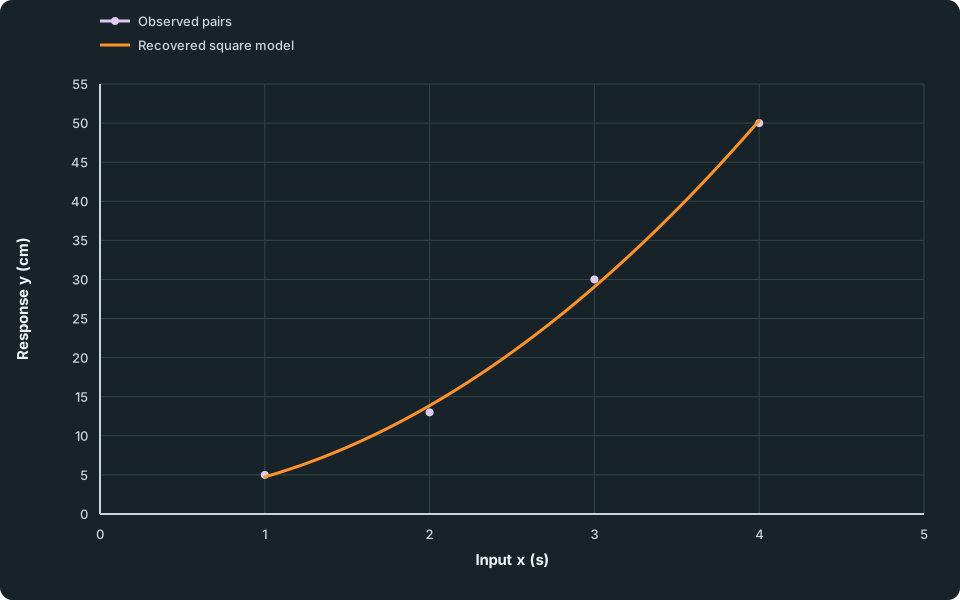
Four circular observations rise at an increasing rate as x increases. The fitted square-model curve follows this upward bend. Only the observed input interval from 1 to 4 seconds is drawn.
Scroll across the figure to read all labels.
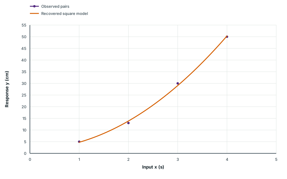
View figure data
| Series | Input x (s) | Response y (cm) |
|---|---|---|
| Observed pairs | 1.00 | 5.000 |
| Observed pairs | 2.00 | 13.000 |
| Observed pairs | 3.00 | 30.000 |
| Observed pairs | 4.00 | 50.000 |
| Recovered square model | 1.00 | 4.748 |
| Recovered square model | 1.05 | 5.060 |
| Recovered square model | 1.10 | 5.386 |
| Recovered square model | 1.15 | 5.728 |
| Recovered square model | 1.20 | 6.085 |
| Recovered square model | 1.25 | 6.457 |
| Recovered square model | 1.30 | 6.845 |
| Recovered square model | 1.35 | 7.247 |
| Recovered square model | 1.40 | 7.665 |
| Recovered square model | 1.45 | 8.098 |
| Recovered square model | 1.50 | 8.547 |
| Recovered square model | 1.55 | 9.010 |
| Recovered square model | 1.60 | 9.489 |
| Recovered square model | 1.65 | 9.982 |
| Recovered square model | 1.70 | 10.491 |
| Recovered square model | 1.75 | 11.016 |
| Recovered square model | 1.80 | 11.555 |
| Recovered square model | 1.85 | 12.109 |
| Recovered square model | 1.90 | 12.679 |
| Recovered square model | 1.95 | 13.264 |
| Recovered square model | 2.00 | 13.864 |
| Recovered square model | 2.05 | 14.480 |
| Recovered square model | 2.10 | 15.110 |
| Recovered square model | 2.15 | 15.756 |
| Recovered square model | 2.20 | 16.417 |
| Recovered square model | 2.25 | 17.093 |
| Recovered square model | 2.30 | 17.784 |
| Recovered square model | 2.35 | 18.491 |
| Recovered square model | 2.40 | 19.213 |
| Recovered square model | 2.45 | 19.949 |
| Recovered square model | 2.50 | 20.702 |
| Recovered square model | 2.55 | 21.469 |
| Recovered square model | 2.60 | 22.251 |
| Recovered square model | 2.65 | 23.049 |
| Recovered square model | 2.70 | 23.862 |
| Recovered square model | 2.75 | 24.690 |
| Recovered square model | 2.80 | 25.533 |
| Recovered square model | 2.85 | 26.392 |
| Recovered square model | 2.90 | 27.265 |
| Recovered square model | 2.95 | 28.154 |
| Recovered square model | 3.00 | 29.058 |
| Recovered square model | 3.05 | 29.977 |
| Recovered square model | 3.10 | 30.912 |
| Recovered square model | 3.15 | 31.861 |
| Recovered square model | 3.20 | 32.826 |
| Recovered square model | 3.25 | 33.806 |
| Recovered square model | 3.30 | 34.801 |
| Recovered square model | 3.35 | 35.812 |
| Recovered square model | 3.40 | 36.837 |
| Recovered square model | 3.45 | 37.878 |
| Recovered square model | 3.50 | 38.934 |
| Recovered square model | 3.55 | 40.005 |
| Recovered square model | 3.60 | 41.092 |
| Recovered square model | 3.65 | 42.193 |
| Recovered square model | 3.70 | 43.310 |
| Recovered square model | 3.75 | 44.442 |
| Recovered square model | 3.80 | 45.589 |
| Recovered square model | 3.85 | 46.751 |
| Recovered square model | 3.90 | 47.929 |
| Recovered square model | 3.95 | 49.122 |
| Recovered square model | 4.00 | 50.329 |
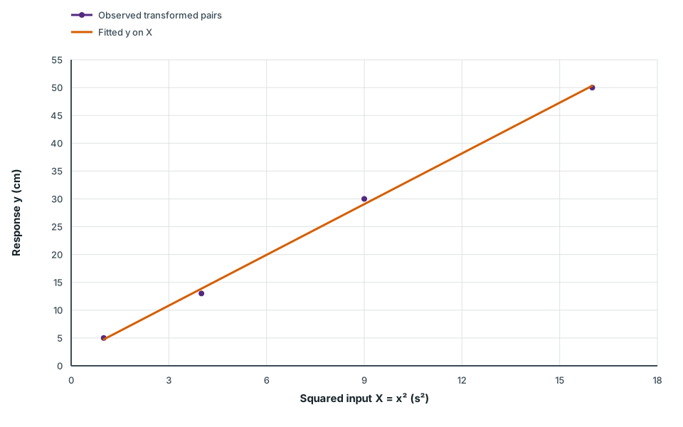
The same observations against squared input
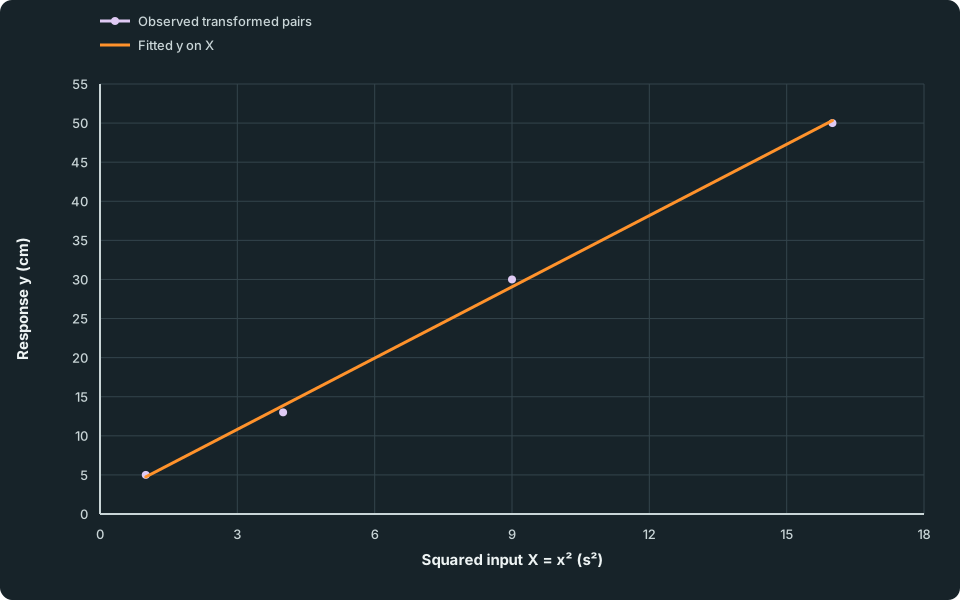
The same four response observations now lie close to a straight increasing line when plotted against squared input. Their vertical residuals are still measured in centimetres because only the input axis has changed.
Scroll across the figure to read all labels.
View figure data
| Series | Squared input X = x² (s²) | Response y (cm) |
|---|---|---|
| Observed transformed pairs | 1 | 5.000 |
| Observed transformed pairs | 4 | 13.000 |
| Observed transformed pairs | 9 | 30.000 |
| Observed transformed pairs | 16 | 50.000 |
| Fitted y on X | 1 | 4.748 |
| Fitted y on X | 16 | 50.329 |
Only the input changed, so vertical residuals still measure y discrepancies in cm. The sum of their squares is approximately 1.80620 cm² for the square-input fit, compared with 37.8 cm² for a direct straight-line y-on-x fit to these same observations. These totals are on the same response scale and can be compared for that fitting criterion. The better fit to four observations supports consideration of the square model; it does not establish a physical law or a reliable extrapolation.
The fitted intercept is an estimated parameter, not an observed y at x = 0: the measurements cover only 1 to 4 s. Squaring also loses the original input’s sign. Keep the original domain when interpreting a transformed plot or recovering an input.
A reciprocal input has its own domain and units
For a proposed model y = a + b/x, define X = 1/x and fit y on X, with x ≠ 0. A straight-line gradient in this plot belongs to reciprocal input, not to x itself. If x is in seconds and y in centimetres, X has unit s⁻¹ and b has unit cm·s.
Check your understanding 1 Name the input that was actually fitted
For measurements with 2 ≤ x ≤ 8 seconds and y in cm, a fit against X = 1/x gives ŷ = 3 + 12X. Recover the model in x, predict y at x = 3 s, and state the coefficient units. Explain what fails at x = 0 and whether evaluating a formula at an input outside the calibrated range establishes a reliable prediction.
Show answer
The model is y hat = 3 + 12/x. At x = 3 s, the transformed input is 1/3 s⁻¹ and the prediction is 7 cm. The intercept is 3 cm and the reciprocal coefficient is 12 cm·s, so dividing it by x gives cm again.
At x = 0 the reciprocal input is undefined. At another input outside 2 to 8 s, an algebraic value alone does not supply calibration evidence. Even a valid mathematical domain is not a guarantee that the empirical model applies throughout it.
A transformed response needs its own inverse
Transforming the response changes what the fitted line predicts. If Y = y², the fitted value is a square, not y itself. Recovering y needs a square root and the original variable’s stated sign or domain. The squared equation alone does not choose between the two roots. A negative fitted Y has no real square-root recovery.
If Y = 1/y, recover the original response with y = 1/Ŷ. This is undefined when the fitted Ŷ is zero. In each case residuals for the least-squares fit are discrepancies in Y, rather than in original y. Do not compare their squared totals as though the response scale had stayed unchanged.
Check your understanding 2 Recover the stated original response
A model is fitted to (x,y) = (1,−1), (4,−2), (9,−3) using Y = y² as response and x as input. The original response is known to be nonpositive. Find the fitted intercept and gradient, then predict original y at x = 4. Explain what fails at x = −1, and what must be considered before interpreting its computed prediction at x = 16.
Separately, (x,y) = (1,2), (2,1), (4,0.5) gives the fitted reciprocal-response line Ŷ = 0.5x with Y = 1/y. Predict original y at x = 3. On which response scale are its fitting residuals measured?
Show answer
The squared responses are 1, 4 and 9, so the fit is Ŷ = x: intercept 0 and gradient 1. At x = 4 it predicts Y = 4, and the stated nonpositive branch gives y = −2. Taking the positive root would ignore the original response’s domain. At x = −1 the fitted square would be negative, so it has no real original-response prediction. At x = 16 the model gives y = −4, but this extrapolates beyond the observed x range 1 to 9; the calculation alone does not establish reliability there.
For the reciprocal-response model, x = 3 gives Ŷ = 1.5, hence y hat = 1/1.5 = 2/3. Its fitting residuals are observed 1/y minus fitted 1/y. They are not original y residuals. Both models need the inverse transformation before reporting a prediction in the original response variable, and neither computation establishes the model’s suitability or a causal relationship.
Logging the output changes the fitted error scale
For a proposed power model y = axⁿ with x > 0 and a > 0, take logs and define X = ln x and Y = ln y. Then
Fit Y on X. If the fitted line is Y hat = A + nX, recover the model prediction as
The gradient is the exponent n, while the intercept is ln a, not a. These logarithmic examples use positive dimensionless x and y. For measured quantities, specify fixed reference units and form the corresponding dimensionless numerical ratios before taking logs.
For an exponential model y = kb^x with k > 0 and b > 0, instead fit ln y against x, leaving the input unlogged. From Y hat = A + Bx, recover k = eᴬ and b = eᴮ, so y hat = e^A(e^B)^x. A power model and an exponential model use different input columns.
The log base also belongs to the fit. If Y = log₁₀ y, recover an intercept factor with 10ᴬ, not eᴬ. A base-10 gradient B in a log-output-against-x fit gives a factor 10ᴮ for an increase of one in x. Do not change the inverse base while keeping the original fitted coefficients.
Check your understanding 3 Recover the original prediction
A fit using natural logs gives ln y = 0.5 + 2 ln x and was calibrated for 1 ≤ x ≤ 5. Predict y at x = 3 to three significant figures, and state the model form. Explain why substituting x = −3 or x = 8 into the recovered formula needs more care than simply obtaining a numerical output.
Show answer
The fitted model is y hat = e^(0.5)x², so at x = 3 the prediction is 9e^(0.5) ≈ 14.8384914, or 14.8 to three significant figures. The slope 2 is an exponent because both original variables were logged.
Although the recovered algebraic expression can be evaluated at −3, ln x was defined only for x > 0 in the fitted model. The positive output from squaring −3 does not extend that log-model domain. At x = 8 the logs exist, but this is extrapolation beyond the original calibration interval 1 to 5. Neither case gains empirical support just because the final formula returns a value.
The fit minimises squared residuals in log output, not in original y. A log residual is ln y-Y hat = ln(y/y hat), so it measures a multiplicative discrepancy. The same log discrepancy can correspond to very different absolute errors at small and large original responses.
Back-transforming a fitted log value gives a model prediction on the original scale. It does not automatically give the original-scale conditional mean. For a simple illustration, two equally likely positive responses 1 and 9 have average log ln 3; exponentiating gives 3, while their arithmetic mean is 5. Averaging and exponentiating do not generally commute. Interpreting a back-transformed fit as a mean response requires further justification about its error model.
A larger transformed r is not a universal model verdict
Inspect the transformed scatter as well as its r. A plausible model should have residuals without an unexplained systematic pattern on the scale being fitted. A high transformed r alone does not settle model choice, mechanism, prediction quality or the range over which the model is useful.
If only the input is transformed, original y residuals retain their units, as in the square-input example. If the response is logged, its residual scale changes. Numerically comparing a squared-error total in cm² with one in squared log ratios does not rank original-scale prediction errors.
Check your understanding 4 Compare predictions on a stated scale
Model A is fitted to y, while model B is fitted to ln y and then back-transformed. A claim says B must predict original y better because its fitting sum of squared log errors is numerically smaller than A’s sum of squared y errors. Assess that claim.
For two additional observations, the original-scale predictions are:
| Observed y | A prediction | B prediction |
|---|---|---|
| 10 | 9 | 12 |
| 100 | 90 | 110 |
Calculate each model’s sum of squared errors on this original-scale table. State what that comparison supports and what it does not establish.
Show answer
The fitting totals use different response scales and are not directly comparable merely by their numerical sizes. On the additional observations, A has errors 1 and 10, so its squared-error total is 101. B has errors −2 and −10, giving 104.
A has the smaller squared error on this original-scale table. This limited comparison does not establish a universally better model or performance on every future observation. A different prediction purpose or loss criterion can emphasise different discrepancies. The model’s setting and the stated response-error scale must accompany the comparison.
Record enough to reproduce a transformed fit: the paired variables and their units, transformation and log base, columns entered, fitted coefficients, recovered model and original calibration range. Retain full coefficient precision in calculations. A well-fitted transformed line does not remove original-domain, range or prediction-meaning checks.
Try it yourself 1
Use a calibration on a logarithmic response scale
Problem
A calibration uses t, the numerical elapsed time in hours, and a positive dimensionless response y. Measurements cover 0 ≤ t ≤ 4. A linear fit with input t and response Y = log₁₀ y gives Ŷ = 0.3 + 0.2t.
Recover the original model and predict y at t = 2.5 to three significant figures. Find its multiplicative change for an extra hour and the time at which the fitted response reaches y = 10. Assess use of the same fit at t = 10. If Ŷ is interpreted as a fitted mean log response, explain whether back-transforming it automatically estimates the mean of the original response.
Write your answer, then compare it with the solution
Hints
Hint 1
Read both axis definitions before inverting
Identify which quantity was logged, which log base was used and which input stayed unchanged. For the requested response threshold, put its logged value into the fitted line before checking the corresponding original time range.
Show full solution
Recover a model from the fitted log response
Method
Invert the base-10 response transformation, leaving t as the input.Reason
The input is time, not log time, so this is an exponential rather than a power model in t. Later solving its fitted response for a target is inversion of this calibration model, not a separate time-on-response regression.Working
Answer
y hat = 10^(0.3 + 0.2t) = 10^(0.3)(10^(0.2))^t. At t = 2.5, the fitted log response is 0.8 and the back-transformed prediction is 10^(0.8) ≈ 6.30957344, or 6.31 to three significant figures.Interpret a one-hour change and solve for the response threshold
Method
Use the exponential factor for time increments and the logged threshold for the inverse estimate.Reason
A gradient of 0.2 changes log₁₀ y by 0.2 per hour; it does not add 0.2 directly to y.Working
Answer
For an extra hour, the fitted original response is multiplied by 10^(0.2) ≈ 1.58489319, an increase of about 58.5%. For y = 10, log₁₀ y = 1, so 1 = 0.3 + 0.2t gives t = 3.5 hours. Both 2.5 and 3.5 lie within the original 0-to-4-hour calibration range.Keep the prediction's range and meaning explicit
Method
Distinguish a computed extrapolation and back-transformed prediction from a supported original-scale mean.Reason
The fit was calibrated on a finite range and minimises log-scale, rather than original-scale, squared residuals.Working
Answer
At t = 10 the formula gives 10^(2.3) ≈ 199.526, but this extrapolates well beyond 4 hours and has no reliability guarantee from the fitted data alone. Exponentiating a fitted mean log response does not in general produce the mean original response. Report the original-scale value as the back-transformed model prediction unless further error-model assumptions justify a mean interpretation.
Quick check
Compare your axis definitions, inverse base, model form, change factor and calibration range separately. Returning to the original scale also requires returning to the original question: a prediction, an arithmetic mean and a guarantee for an individual are different claims.
Keep track of this lesson
Mark the lesson done when you have worked through it.
Lesson progress is optional and kept on this device.
Loading lesson controls…
Your lesson mark records your own study. Checks are kept separately in My Learning.