On this page
Loading guide controls…
Continue lessonNew guided lessons are not available yet.
Guided lesson options
You stopped at:
ContinueRevision Mode is on. Questions and activities are hidden.
The linked question or activity is hidden by Revision Mode.
With a small sample from a normal population whose variance is unknown, replacing σ by the sample estimate s changes the distribution of the test statistic: it is no longer standard normal but a t-distribution with heavier tails. This lesson carries out a one-sample t-test in the form 9649 expects, builds confidence intervals for a mean and for a proportion, connects an interval to a two-tailed test, and states precisely what “95% confidence” does and does not mean.
Estimating the variance changes the distribution
For a random sample of size n from a normal population with mean μ, the sample mean X bar is normal with variance σ²/n. When σ² is unknown we replace it by the unbiased estimate
The resulting statistic
follows a t-distribution with n-1 degrees of freedom, tₙ₋₁. It is symmetric like the standard normal but has heavier tails, because s itself varies from sample to sample; as n grows, it approaches the normal. For a small sample the normal-population assumption is essential; for a large sample, the central limit theorem lets the normal distribution be used instead.
Heavier tails when variance is estimated
The solid t distribution with 7 degrees of freedom has density about 0.385 at zero and 0.014 at 3. The dashed standard normal has density about 0.399 at zero and 0.00443 at 3.
Scroll across to read every label.
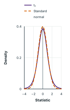
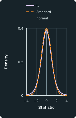
Figure data
This table is included in print while it is open.
| Statistic | t₇ | Standard normal |
|---|---|---|
| -4.00 | 0.003303 | 0.0001338 |
| -3.95 | 0.003542 | 0.0001633 |
| -3.90 | 0.003799 | 0.0001987 |
| -3.85 | 0.004076 | 0.0002411 |
| -3.80 | 0.004375 | 0.0002919 |
| -3.75 | 0.004697 | 0.0003526 |
| -3.70 | 0.005044 | 0.0004248 |
| -3.65 | 0.005419 | 0.0005105 |
| -3.60 | 0.005824 | 0.0006119 |
| -3.55 | 0.006260 | 0.0007317 |
| -3.50 | 0.006732 | 0.0008727 |
| -3.45 | 0.007240 | 0.0010383 |
| -3.40 | 0.007790 | 0.0012322 |
| -3.35 | 0.008383 | 0.0014587 |
| -3.30 | 0.009024 | 0.0017226 |
| -3.25 | 0.009716 | 0.0020290 |
| -3.20 | 0.010464 | 0.0023841 |
| -3.15 | 0.011272 | 0.0027943 |
| -3.10 | 0.012144 | 0.0032668 |
| -3.05 | 0.013087 | 0.0038098 |
| -3.00 | 0.014105 | 0.0044318 |
| -2.95 | 0.015204 | 0.0051426 |
| -2.90 | 0.016392 | 0.0059525 |
| -2.85 | 0.017675 | 0.0068728 |
| -2.80 | 0.019059 | 0.0079155 |
| -2.75 | 0.020554 | 0.0090936 |
| -2.70 | 0.022167 | 0.0104209 |
| -2.65 | 0.023908 | 0.0119122 |
| -2.60 | 0.025785 | 0.0135830 |
| -2.55 | 0.027809 | 0.0154493 |
| -2.50 | 0.029990 | 0.0175283 |
| -2.45 | 0.032340 | 0.0198374 |
| -2.40 | 0.034869 | 0.0223945 |
| -2.35 | 0.037591 | 0.0252182 |
| -2.30 | 0.040517 | 0.0283270 |
| -2.25 | 0.043661 | 0.0317397 |
| -2.20 | 0.047037 | 0.0354746 |
| -2.15 | 0.050658 | 0.0395500 |
| -2.10 | 0.054538 | 0.0439836 |
| -2.05 | 0.058693 | 0.0487920 |
| -2.00 | 0.063135 | 0.0539910 |
| -1.95 | 0.067881 | 0.0595947 |
| -1.90 | 0.072943 | 0.0656158 |
| -1.85 | 0.078335 | 0.0720649 |
| -1.80 | 0.084070 | 0.0789502 |
| -1.75 | 0.090161 | 0.0862773 |
| -1.70 | 0.096618 | 0.0940491 |
| -1.65 | 0.103450 | 0.1022649 |
| -1.60 | 0.110665 | 0.1109208 |
| -1.55 | 0.118269 | 0.1200090 |
| -1.50 | 0.126263 | 0.1295176 |
| -1.45 | 0.134648 | 0.1394306 |
| -1.40 | 0.143420 | 0.1497275 |
| -1.35 | 0.152573 | 0.1603833 |
| -1.30 | 0.162093 | 0.1713686 |
| -1.25 | 0.171965 | 0.1826491 |
| -1.20 | 0.182169 | 0.1941861 |
| -1.15 | 0.192676 | 0.2059363 |
| -1.10 | 0.203456 | 0.2178522 |
| -1.05 | 0.214470 | 0.2298821 |
| -1.00 | 0.225675 | 0.2419707 |
| -0.95 | 0.237020 | 0.2540591 |
| -0.90 | 0.248450 | 0.2660852 |
| -0.85 | 0.259903 | 0.2779849 |
| -0.80 | 0.271313 | 0.2896916 |
| -0.75 | 0.282606 | 0.3011374 |
| -0.70 | 0.293708 | 0.3122539 |
| -0.65 | 0.304539 | 0.3229724 |
| -0.60 | 0.315016 | 0.3332246 |
| -0.55 | 0.325055 | 0.3429439 |
| -0.50 | 0.334573 | 0.3520653 |
| -0.45 | 0.343487 | 0.3605270 |
| -0.40 | 0.351715 | 0.3682701 |
| -0.35 | 0.359181 | 0.3752403 |
| -0.30 | 0.365812 | 0.3813878 |
| -0.25 | 0.371543 | 0.3866681 |
| -0.20 | 0.376316 | 0.3910427 |
| -0.15 | 0.380081 | 0.3944793 |
| -0.10 | 0.382799 | 0.3969525 |
| -0.05 | 0.384442 | 0.3984439 |
| 0.00 | 0.384991 | 0.3989423 |
| 0.05 | 0.384442 | 0.3984439 |
| 0.10 | 0.382799 | 0.3969525 |
| 0.15 | 0.380081 | 0.3944793 |
| 0.20 | 0.376316 | 0.3910427 |
| 0.25 | 0.371543 | 0.3866681 |
| 0.30 | 0.365812 | 0.3813878 |
| 0.35 | 0.359181 | 0.3752403 |
| 0.40 | 0.351715 | 0.3682701 |
| 0.45 | 0.343487 | 0.3605270 |
| 0.50 | 0.334573 | 0.3520653 |
| 0.55 | 0.325055 | 0.3429439 |
| 0.60 | 0.315016 | 0.3332246 |
| 0.65 | 0.304539 | 0.3229724 |
| 0.70 | 0.293708 | 0.3122539 |
| 0.75 | 0.282606 | 0.3011374 |
| 0.80 | 0.271313 | 0.2896916 |
| 0.85 | 0.259903 | 0.2779849 |
| 0.90 | 0.248450 | 0.2660852 |
| 0.95 | 0.237020 | 0.2540591 |
| 1.00 | 0.225675 | 0.2419707 |
| 1.05 | 0.214470 | 0.2298821 |
| 1.10 | 0.203456 | 0.2178522 |
| 1.15 | 0.192676 | 0.2059363 |
| 1.20 | 0.182169 | 0.1941861 |
| 1.25 | 0.171965 | 0.1826491 |
| 1.30 | 0.162093 | 0.1713686 |
| 1.35 | 0.152573 | 0.1603833 |
| 1.40 | 0.143420 | 0.1497275 |
| 1.45 | 0.134648 | 0.1394306 |
| 1.50 | 0.126263 | 0.1295176 |
| 1.55 | 0.118269 | 0.1200090 |
| 1.60 | 0.110665 | 0.1109208 |
| 1.65 | 0.103450 | 0.1022649 |
| 1.70 | 0.096618 | 0.0940491 |
| 1.75 | 0.090161 | 0.0862773 |
| 1.80 | 0.084070 | 0.0789502 |
| 1.85 | 0.078335 | 0.0720649 |
| 1.90 | 0.072943 | 0.0656158 |
| 1.95 | 0.067881 | 0.0595947 |
| 2.00 | 0.063135 | 0.0539910 |
| 2.05 | 0.058693 | 0.0487920 |
| 2.10 | 0.054538 | 0.0439836 |
| 2.15 | 0.050658 | 0.0395500 |
| 2.20 | 0.047037 | 0.0354746 |
| 2.25 | 0.043661 | 0.0317397 |
| 2.30 | 0.040517 | 0.0283270 |
| 2.35 | 0.037591 | 0.0252182 |
| 2.40 | 0.034869 | 0.0223945 |
| 2.45 | 0.032340 | 0.0198374 |
| 2.50 | 0.029990 | 0.0175283 |
| 2.55 | 0.027809 | 0.0154493 |
| 2.60 | 0.025785 | 0.0135830 |
| 2.65 | 0.023908 | 0.0119122 |
| 2.70 | 0.022167 | 0.0104209 |
| 2.75 | 0.020554 | 0.0090936 |
| 2.80 | 0.019059 | 0.0079155 |
| 2.85 | 0.017675 | 0.0068728 |
| 2.90 | 0.016392 | 0.0059525 |
| 2.95 | 0.015204 | 0.0051426 |
| 3.00 | 0.014105 | 0.0044318 |
| 3.05 | 0.013087 | 0.0038098 |
| 3.10 | 0.012144 | 0.0032668 |
| 3.15 | 0.011272 | 0.0027943 |
| 3.20 | 0.010464 | 0.0023841 |
| 3.25 | 0.009716 | 0.0020290 |
| 3.30 | 0.009024 | 0.0017226 |
| 3.35 | 0.008383 | 0.0014587 |
| 3.40 | 0.007790 | 0.0012322 |
| 3.45 | 0.007240 | 0.0010383 |
| 3.50 | 0.006732 | 0.0008727 |
| 3.55 | 0.006260 | 0.0007317 |
| 3.60 | 0.005824 | 0.0006119 |
| 3.65 | 0.005419 | 0.0005105 |
| 3.70 | 0.005044 | 0.0004248 |
| 3.75 | 0.004697 | 0.0003526 |
| 3.80 | 0.004375 | 0.0002919 |
| 3.85 | 0.004076 | 0.0002411 |
| 3.90 | 0.003799 | 0.0001987 |
| 3.95 | 0.003542 | 0.0001633 |
| 4.00 | 0.003303 | 0.0001338 |
Worked example 1
Are the packets underweight?
Worked example 1
Are the packets underweight?
Packets are labelled 500 g. The masses, in grams, of a random sample of 8 packets are
Assuming masses are normally distributed, test at the 5% level whether the mean mass is less than 500 g.
Show full solutionHide solution
Hypotheses and statistics
Method
H₀:μ = 500 against H₁:μ < 500, a one-tailed test.Reason
The claim to be tested is a shortfall, and σ is unknown with n small, so use t₇.Working
Answer
x bar = 3982/8 = 497.75, and s² = 1/7∑(xᵢ-x bar)² = 111/14 ≈ 7.929, so s ≈ 2.816.
Test statistic and decision
Method
t = (497.75-500)/(2.816/square root of 8) ≈ -2.260.Reason
The one-tailed 5% critical value of t₇ is -1.895.Working
Answer
Since -2.260 < -1.895 (equivalently, the p-value 0.029 is below 0.05), reject H₀. There is sufficient evidence at the 5% level that the mean mass of packets is less than 500 g.
Quick check
Using z_(0.05) = -1.645 would understate how far t must go: with only 7 degrees of freedom the tails are heavier. The conclusion is about the population mean, stated in context and with the level; it does not prove the claim.
Confidence intervals and their link to tests
A 95% confidence interval for μ from a small sample of a normal population is
where tₙ₋₁ is the two-tailed 5% critical value. Other cases use the same pattern: x bar ± z σ/square root of n when σ is known for a normal population; x bar ± z s/square root of n for a large sample from any population; and p hat ± z square root of (p hat (1-p hat)/n) for a proportion from a large sample.
A two-tailed test at the 5% level rejects H₀:μ = μ₀ exactly when μ₀ lies outside the 95% interval built from the same data.
Check your understanding 1
One sample, two conclusions
Check your understanding 1
One sample, two conclusions
For the packet data, with two-tailed t₇ critical value 2.365, find a 95% confidence interval for the mean mass. What does it say about a two-tailed 5% test of μ = 500, and why does this differ from the one-tailed result?
Show answerHide answer
497.75±2.365 × 2.816/(square root of 8) = 497.75±2.354, giving (495.40, 500.10). It contains 500, so a two-tailed 5% test would not reject μ = 500: |t| = 2.260 < 2.365. The one-tailed test puts all 5% in the lower tail, so its critical value 1.895 is smaller. The choice of tail must come from the question asked before seeing the data.
Spot the mistake 1
What 95% means
Spot the mistake 1
What 95% means
A student writes: “There is a 95% probability that the true mean mass lies between 495.40 g and 500.10 g.” Explain what is wrong and give a correct interpretation.
Write your answer, then compare it with the solution
Show full solutionHide solution
Locate the randomness
Method
The true mean is fixed; it is the interval that varies from sample to sample.Reason
Once calculated, this particular interval either contains μ or it does not.Working
Answer
Correctly: if many random samples of 8 packets were taken and an interval calculated in this way from each, about 95% of those intervals would contain the true mean mass.
Common mistake
The 95% describes the long-run success rate of the method. It also depends on the model assumptions, here a normal population and a random sample.
Common mistakes
- Using a z critical value when σ is unknown and the sample is small; the t value with n-1 degrees of freedom is larger.
- Dividing by n instead of n-1 in s², or using s instead of s/(square root of n) as the standard error.
- Forgetting to state that the population is assumed normal for a small-sample t-test.
- Comparing a two-tailed interval with a one-tailed test at the same level.
- Saying there is a 95% probability that μ lies in a particular calculated interval.
Before you move on
Check your understanding 2
An interval for a proportion
Check your understanding 2
An interval for a proportion
In a random sample of 400 residents, 92 support a proposed bus route. Find an approximate 95% confidence interval for the proportion p of all residents who support it, giving the bounds to three decimal places. Then decide whether the interval supports a claim that a quarter of residents support the route.
Show answerHide answer
The sample is large, so the sample proportion p hat = 92/400 = 0.23 is approximately normal:
giving (0.189, 0.271). The value 0.25 lies inside, so a two-tailed test at the 5% level would not reject p = 0.25: the data are consistent with a quarter of residents supporting the route, though they do not prove it.
Paired and two-sample tests continue in Paired and two-sample tests, and χ² tests in χ² tests.
Loading reading progress…
Lesson done
- Monday
- Tuesday
- Wednesday
- Thursday
- Friday
- Saturday
- Sunday
Checking learning on this device…
Change goal
Progress options
Loading questions…