Linearise power and exponential models
Choose transformed axes, recover power or exponential constants and test the model against original data and domain limits.
More
Offline pages
Saved on this device only. Connect at least once every 30 days to confirm Premium. Sign-out or a change of account removes saved copies.
Find this activity in your course
On this page
You stopped at:
ContinueRevision Mode is on. Questions and activities are hidden.
Change the variables before reading the gradient
A curved relationship can become a straight line when we plot different variables. The gradient and intercept belong to the labelled axes, not automatically to x and y. Rewrite the proposed relationship as Y = mX + c, name X and Y, then match coefficients.
Recall that log ₁₀y = q means y = 10^q, while ln y = q means y = e^q. Taking a logarithm and undoing it are different operations. All x and y values in the examples below are dimensionless; for measured quantities, first fix the units used for their numerical values.
A power model becomes linear in two logarithms
For y = axⁿ with a > 0 and x > 0, y is positive. Taking base-ten logarithms gives
With X = log ₁₀x and Y = log ₁₀y, this is a straight line of gradient n and vertical intercept log ₁₀a. The intercept is not a itself.
Suppose the transformed graph passes through (X,Y) = (0,1), (1,3) and (2,5). Its gradient is (5 − 1)/(2 − 0) = 2 and its intercept is 1. Therefore n = 2 and a = 10¹ = 10, giving y = 10x².
| Original x | Original y | X = log₁₀x | Y = log₁₀y |
|---|---|---|---|
| 1 | 10 | 0 | 1 |
| 10 | 1000 | 1 | 3 |
| 100 | 100000 | 2 | 5 |
The transformed intercept at X = 0 corresponds to x = 1, because log₁₀1 = 0. It is not the original y-intercept at x = 0. Check the recovered model on the original scale: x = 10 gives y = 10 × 10² = 1000.
A power model is straight on two logarithmic variables
An increasing straight line on transformed coordinates, with marked points (0,1), (1,3) and (2,5). The horizontal axis is log₁₀x, rather than x, and the vertical axis is log₁₀y. Its vertical intercept is one and gradient two.
Scroll across the figure to read all labels.
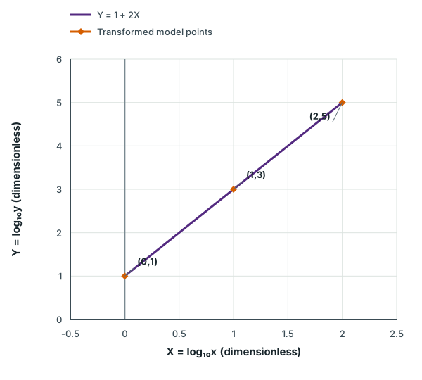
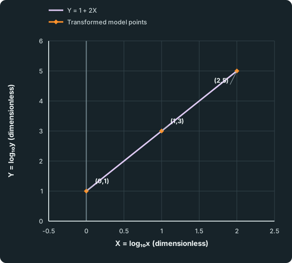
View figure data
| Series | X = log₁₀x (dimensionless) | Y = log₁₀y (dimensionless) |
|---|---|---|
| Y = 1 + 2X | 0 | 1 |
| Y = 1 + 2X | 2 | 5 |
| Transformed model points | 0 | 1 |
| Transformed model points | 1 | 3 |
| Transformed model points | 2 | 5 |
Using natural logarithms instead gives ln y = ln a + n ln x. The slope is still n when both axes use the same logarithm base, but the intercept now needs a = eᶜ. For a line with gradient 1.5 and intercept 0.7 on these natural-log axes, y = e^(0.7)x^(1.5). The coefficient is e^0.7, rather than 0.7.
Check your understanding 1 Read the transformed origin correctly
A graph of ln y against ln x has gradient −1/2 and vertical intercept ln 6. Recover the power model, find y at x = 4 and explain which original x-value corresponds to that transformed intercept.
Show answer
The line is ln y = ln 6-1/2 ln x, so y = 6x^(-1/2) = 6/square root of x for x > 0. At x = 4, y = 3. The transformed intercept has ln x = 0, hence x = 1 and y = 6. It does not supply a value at x = 0, where this model is undefined. A negative slope here means a negative power, not negative y-values.
An exponential model leaves the input unlogged
For y = kb^x with k > 0 and b > 0, taking base-ten logarithms gives
Choose X = x, rather than log₁₀x, and Y = log₁₀y. The line has gradient log₁₀b and intercept log₁₀k. Both constants need an inverse logarithm: k = 10ᶜ and b = 10ᵐ. A negative gradient gives 0 < b < 1, rather than a negative base.
Suppose this graph passes through (0,2), (2,1) and (4,0). Its gradient is −1/2 and intercept 2. Thus k = 100 and b = 10^(-1/2), giving y = 100(10^(-1/2))^x.
| x, unchanged | y | Y = log₁₀y |
|---|---|---|
| 0 | 100 | 2 |
| 2 | 10 | 1 |
| 4 | 1 | 0 |
At x = 2, the model gives 100 × 10⁻¹ = 10, agreeing with the original value. Here the transformed intercept really does occur at x = 0, since the horizontal axis was not logged.
An exponential model leaves x unchanged
A decreasing straight line through marked transformed points (0,2), (2,1) and (4,0). The horizontal axis is the original input x; only the vertical variable is log₁₀y. Its gradient is minus one half and vertical intercept two.
Scroll across the figure to read all labels.
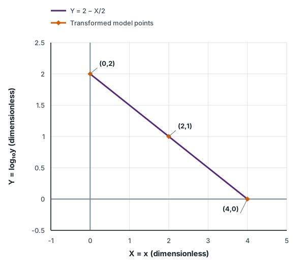
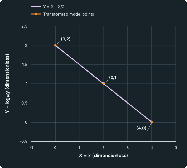
View figure data
| Series | X = x (dimensionless) | Y = log₁₀y (dimensionless) |
|---|---|---|
| Y = 2 − X/2 | 0 | 2 |
| Y = 2 − X/2 | 4 | 0 |
| Transformed model points | 0 | 2 |
| Transformed model points | 2 | 1 |
| Transformed model points | 4 | 0 |
Natural logarithms work too: ln y = ln k + x ln b. A line of gradient −0.4 and intercept 2 gives y = e²(e^(-0.4))^x, equivalently y = e^(2-0.4x). At x = 5, ln y = 0, so y = 1; substituting in the original exponential confirms it.
Check your understanding 2 Recover the base, not its logarithm
A graph of log₁₀y against x is a line with gradient 0.3 and intercept 1.2. Express y in the form kbˣ and find its value at x = 1, retaining exact powers of ten. Explain why y = 1.2(0.3)ˣ is not the recovered model.
Show answer
log ₁₀y = 1.2 + 0.3x, so k = 10^1.2 and b = 10^0.3. Thus y = 10^(1.2)(10^(0.3))^x, and at x = 1, y = 10^1.5. The proposed model incorrectly uses the logarithms as the constants. It would also decay because 0 < 0.3 < 1, whereas the given positive gradient means log₁₀b > 0 and therefore b > 1.
Check exactly which quantities need logarithms
For a power log–log plot, both x and y must be positive. For an exponential plot of ln y against x, only y is logged: x = 0 or a negative x is allowed. For instance, y = 4(1/2)ˣ gives y = 4 at x = 0 and y = 8 at x = −1; both points are valid on its ln y against x graph. Rejecting them merely because ln x does not exist would apply a transformation that this model never requested.
Neither transformation allows a logarithm of y = 0 or y < 0. Do not silently omit such observations or add an arbitrary constant to make them positive; first reconsider the proposed model or whether a different given relationship is intended. The constant cases also matter: n = 0 gives y = a, while b = 1 gives y = k. The same positive constant data can fit both forms, so straightness alone need not distinguish them.
Other given relationships may need a different substitution. For y = a/x + b with x ≠ 0, set X = 1/x and Y = y. Then Y = aX + b: the gradient is a and intercept b, without any logarithm. For example, y = 3/x + 2 gives points (X,Y) = (1,5), (1/2,7/2), (1/4,11/4), all on Y = 3X + 2. Read and rearrange the relationship rather than selecting a log plot by habit.
Test the recovered model on the original quantities
Two transformed points determine a line, but further observations test whether that line describes the data. Unequal original x-steps are particularly easy to misread: a power model has a fixed y-factor for a fixed multiplication of positive x, while an exponential model has a fixed y-factor for a fixed addition to x.
Real observations may only lie approximately on a transformed line. Use well-separated points on the chosen straight line to estimate its gradient, retain sufficient precision when undoing logarithms, and compare predictions with the original data. This establishes a useful fit, not an exact law or a guarantee outside the observed range.
Try it yourself 1
Choose a model from the data and challenge it
Problem
An ideal data set is proposed to follow either y = axⁿ or y = kbˣ, with positive constants a, k and b:
| x | 1 | 2 | 4 | 8 |
|---|---|---|---|---|
| y | 10 | 5 | 2.5 | 1.25 |
Choose a suitable straight-line plot, state its equation and recover the original model. A proposal says that halving y proves an exponential model and fits y = 20(1/2)ˣ using the first two observations. Test this claim against an unused point. Predict y at x = 5 and explain how the status of a prediction at x = 16 differs.
Write your answer, then compare it with the solution
Hints
Hint 1
Compare the input steps before interpreting the output factor
The y-values halve each time, but inspect whether the x-values increase by equal differences or equal factors. Choose variables that turn the supported relationship into Y = mX + c, then test a point that was not used to recover the constants.
Show full solution
Identify the relationship and its axes
Method
Compare the factors in x and y across the whole table.Reason
Halving y for doubled x describes a power relationship; it does not establish a constant multiplier for equal additions to x.Working
Answer
Every product xy is 10, so y = 10/x. With X = log₁₀x and Y = log₁₀y, the straight line is Y = 1 − X. For example, x = 1 gives (X,Y) = (0,1), while x = 2 gives (log₁₀2,1 − log₁₀2). The gradient is −1 and intercept 1.Recover and verify the original model
Method
Match the power-model coefficients and return to the original variables.Reason
The slope is n and intercept is log₁₀a on these axes.Working
Answer
n = −1 and a = 10¹ = 10, so y = 10x⁻¹. At x = 4 this gives 2.5, and at x = 8 it gives 1.25, matching the unused observations. A valid alternative is to plot y against 1/x: this gives a line through the origin with gradient 10 and recovers the same model.Test the exponential proposal on unused data
Method
Substitute x = 4 into the competing model.Reason
Agreement at the two points used to construct a model does not establish agreement with the whole data set.Working
Answer
20(1/2)⁴ = 20/16 = 1.25, but the table gives 2.5 at x = 4. The exponential proposal fails. The successive x-differences are 1, 2 and 4, so the repeated halving cannot be interpreted as a multiplier for a fixed additive step.Distinguish prediction within and beyond the data range
Method
Use the recovered model and state the range assumption.Reason
Interpolation lies within the observed x-range; extrapolation extends the model beyond it.Working
Answer
At x = 5, y = 10/5 = 2, an interpolation within 1 ≤ x ≤ 8. At x = 16 the same formula gives 10/16 = 0.625, but this is extrapolation. That value is justified only if the assumed relationship continues; the table alone does not establish it. The positive-domain model does not provide a value at x = 0.
Quick check
Compare the axes, coefficient meanings, original-scale checks and prediction assumptions separately. A different valid straight-line transformation is welcome when its equation recovers the same constants. These are self-review criteria; a straight-looking plot alone does not verify the model.
Keep track of this lesson
Mark the lesson done when you have worked through it.
Lesson progress is optional and kept on this device.
Loading lesson controls…
Your lesson mark records your own study. Checks are kept separately in My Learning.