Graph features and numerical solutions
Interpret graph features, numerical boundaries and model equations, then check precision and feasible solutions.
More
Offline pages
Saved on this device only. Connect at least once every 30 days to confirm Premium. Sign-out or a change of account removes saved copies.
Find this activity in your course
On this page
You stopped at:
ContinueRevision Mode is on. Questions and activities are hidden.
Identify features before trusting a window
A graphing tool can display a function without choosing a useful view of it. Start by identifying features that the rule can check: axis intercepts, symmetry, turning points and asymptotes. Then choose a window showing the relevant parts of the curve.
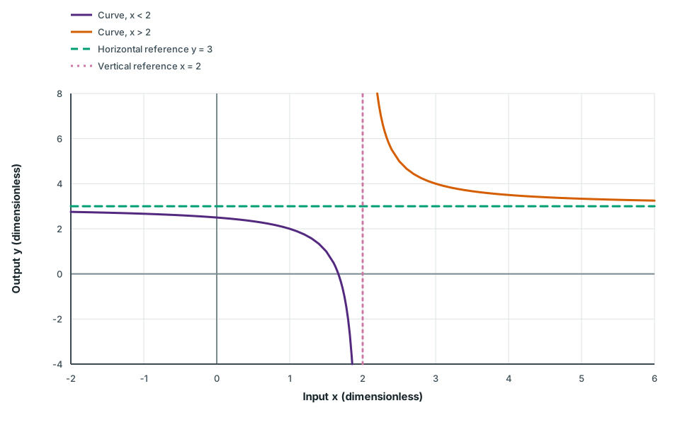
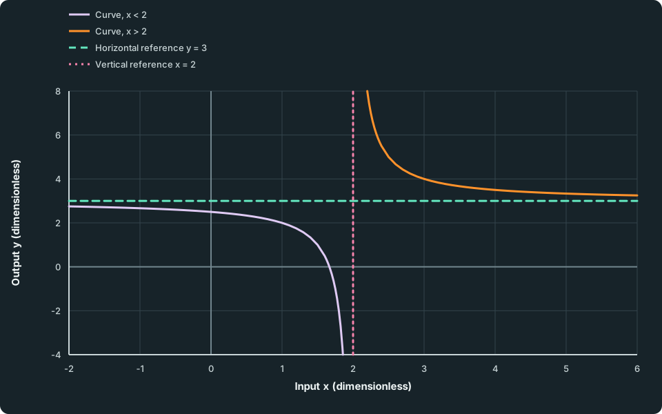
For y = 3 + 1/(x-2), x = 2 is undefined and is a vertical asymptote. Far from x = 2 the reciprocal term approaches zero, giving horizontal asymptote y = 3. At x = 0, y = 2.5, so the y-intercept is (0,2.5). Setting y = 0 gives x = 5/3, so the x-intercept is (5/3,0).
Keep the two branches separate at x = 2
To the left of x = 2 the curve lies below y = 3 and falls steeply near the vertical asymptote. To the right it lies above y = 3 and falls towards that height as x increases. Its intercepts are (0,2.5) and (5/3,0), and the two branches have half-turn symmetry about (2,3).
Scroll across the figure to read all labels.
View figure data
| Series | Input x (dimensionless) | Output y (dimensionless) |
|---|---|---|
| Curve, x < 2 | -2.0000 | 2.75000 |
| Curve, x < 2 | -1.9000 | 2.74359 |
| Curve, x < 2 | -1.8000 | 2.73684 |
| Curve, x < 2 | -1.7000 | 2.72973 |
| Curve, x < 2 | -1.6000 | 2.72222 |
| Curve, x < 2 | -1.5000 | 2.71429 |
| Curve, x < 2 | -1.4000 | 2.70588 |
| Curve, x < 2 | -1.3000 | 2.69697 |
| Curve, x < 2 | -1.2000 | 2.68750 |
| Curve, x < 2 | -1.1000 | 2.67742 |
| Curve, x < 2 | -1.0000 | 2.66667 |
| Curve, x < 2 | -0.9000 | 2.65517 |
| Curve, x < 2 | -0.8000 | 2.64286 |
| Curve, x < 2 | -0.7000 | 2.62963 |
| Curve, x < 2 | -0.6000 | 2.61538 |
| Curve, x < 2 | -0.5000 | 2.60000 |
| Curve, x < 2 | -0.4000 | 2.58333 |
| Curve, x < 2 | -0.3000 | 2.56522 |
| Curve, x < 2 | -0.2000 | 2.54545 |
| Curve, x < 2 | -0.1000 | 2.52381 |
| Curve, x < 2 | 0.0000 | 2.50000 |
| Curve, x < 2 | 0.1000 | 2.47368 |
| Curve, x < 2 | 0.2000 | 2.44444 |
| Curve, x < 2 | 0.3000 | 2.41176 |
| Curve, x < 2 | 0.4000 | 2.37500 |
| Curve, x < 2 | 0.5000 | 2.33333 |
| Curve, x < 2 | 0.6000 | 2.28571 |
| Curve, x < 2 | 0.7000 | 2.23077 |
| Curve, x < 2 | 0.8000 | 2.16667 |
| Curve, x < 2 | 0.9000 | 2.09091 |
| Curve, x < 2 | 1.0000 | 2.00000 |
| Curve, x < 2 | 1.1000 | 1.88889 |
| Curve, x < 2 | 1.2000 | 1.75000 |
| Curve, x < 2 | 1.3000 | 1.57143 |
| Curve, x < 2 | 1.4000 | 1.33333 |
| Curve, x < 2 | 1.5000 | 1.00000 |
| Curve, x < 2 | 1.6000 | 0.50000 |
| Curve, x < 2 | 1.6250 | 0.33333 |
| Curve, x < 2 | 1.6500 | 0.14286 |
| Curve, x < 2 | 1.6750 | -0.07692 |
| Curve, x < 2 | 1.7000 | -0.33333 |
| Curve, x < 2 | 1.7250 | -0.63636 |
| Curve, x < 2 | 1.7500 | -1.00000 |
| Curve, x < 2 | 1.7750 | -1.44444 |
| Curve, x < 2 | 1.8000 | -2.00000 |
| Curve, x < 2 | 1.8250 | -2.71429 |
| Curve, x < 2 | 1.8500 | -3.66667 |
| Curve, x < 2 | 1.8571 | -4.00000 |
| Curve, x > 2 | 2.2000 | 8.00000 |
| Curve, x > 2 | 2.2250 | 7.44444 |
| Curve, x > 2 | 2.2500 | 7.00000 |
| Curve, x > 2 | 2.2750 | 6.63636 |
| Curve, x > 2 | 2.3000 | 6.33333 |
| Curve, x > 2 | 2.3250 | 6.07692 |
| Curve, x > 2 | 2.3500 | 5.85714 |
| Curve, x > 2 | 2.3750 | 5.66667 |
| Curve, x > 2 | 2.4000 | 5.50000 |
| Curve, x > 2 | 2.5000 | 5.00000 |
| Curve, x > 2 | 2.6000 | 4.66667 |
| Curve, x > 2 | 2.7000 | 4.42857 |
| Curve, x > 2 | 2.8000 | 4.25000 |
| Curve, x > 2 | 2.9000 | 4.11111 |
| Curve, x > 2 | 3.0000 | 4.00000 |
| Curve, x > 2 | 3.1000 | 3.90909 |
| Curve, x > 2 | 3.2000 | 3.83333 |
| Curve, x > 2 | 3.3000 | 3.76923 |
| Curve, x > 2 | 3.4000 | 3.71429 |
| Curve, x > 2 | 3.5000 | 3.66667 |
| Curve, x > 2 | 3.6000 | 3.62500 |
| Curve, x > 2 | 3.7000 | 3.58824 |
| Curve, x > 2 | 3.8000 | 3.55556 |
| Curve, x > 2 | 3.9000 | 3.52632 |
| Curve, x > 2 | 4.0000 | 3.50000 |
| Curve, x > 2 | 4.1000 | 3.47619 |
| Curve, x > 2 | 4.2000 | 3.45455 |
| Curve, x > 2 | 4.3000 | 3.43478 |
| Curve, x > 2 | 4.4000 | 3.41667 |
| Curve, x > 2 | 4.5000 | 3.40000 |
| Curve, x > 2 | 4.6000 | 3.38462 |
| Curve, x > 2 | 4.7000 | 3.37037 |
| Curve, x > 2 | 4.8000 | 3.35714 |
| Curve, x > 2 | 4.9000 | 3.34483 |
| Curve, x > 2 | 5.0000 | 3.33333 |
| Curve, x > 2 | 5.1000 | 3.32258 |
| Curve, x > 2 | 5.2000 | 3.31250 |
| Curve, x > 2 | 5.3000 | 3.30303 |
| Curve, x > 2 | 5.4000 | 3.29412 |
| Curve, x > 2 | 5.5000 | 3.28571 |
| Curve, x > 2 | 5.6000 | 3.27778 |
| Curve, x > 2 | 5.7000 | 3.27027 |
| Curve, x > 2 | 5.8000 | 3.26316 |
| Curve, x > 2 | 5.9000 | 3.25641 |
| Curve, x > 2 | 6.0000 | 3.25000 |
| Horizontal reference y = 3 | -2.0000 | 3.00000 |
| Horizontal reference y = 3 | 6.0000 | 3.00000 |
| Vertical reference x = 2 | 2.0000 | -4.00000 |
| Vertical reference x = 2 | 2.0000 | 8.00000 |
The two branches have half-turn symmetry about (2,3): changing an offset from x = 2 to its negative also reverses the offset from y = 3. Both branches are needed to describe the displayed graph. A stroke joining them across the undefined input is not part of the function.
Enter the whole denominator in brackets. The expressions 3 + 1/(x − 2) and 3 + 1/x − 2 describe different functions. A useful window shows both sides of x = 2 and the approach to y = 3; zoom again to inspect the intercepts. A flat-looking segment or a clipped branch is not evidence that the omitted behaviour does not exist.
For this rule the curve never reaches y = 3, since its reciprocal term cannot be zero. Do not turn that example into a universal rule that a horizontal asymptote can never be crossed. For example, y = x/(x² + 1) crosses y = 0 at x = 0 while approaching y = 0 far in either direction.
Intersections solve the original condition
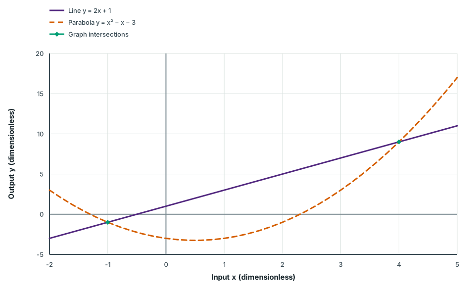
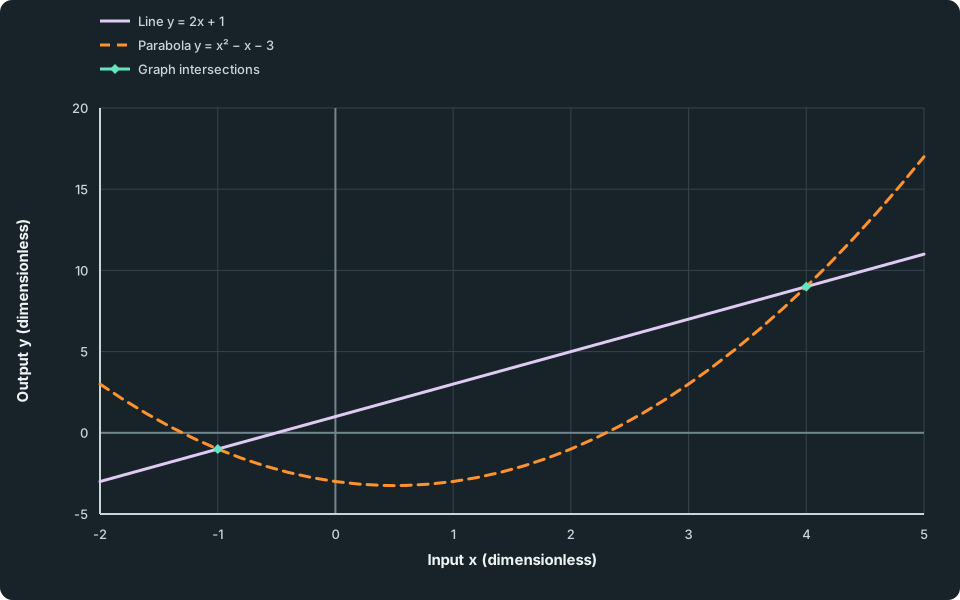
An intersection of two graphs gives a paired solution of their simultaneous equations. Consider the line y = 2x + 1 and parabola y = x² − x − 3. Equating their y-values gives
so x²-3x-4 = (x-4)(x + 1) = 0. The inputs are −1 and 4. Substituting each into the line gives its matching y: the intersection points are (−1,−1) and (4,9). Check those same pairs in the parabola too.
Intersections bound a graphical inequality
The line rises at a constant rate. The parabola turns at (0.5,−3.25), with a vertical symmetry line through x = 0.5. It lies below the line from x = −1 to x = 4 and above it outside that interval within the displayed window.
Scroll across the figure to read all labels.
View figure data
| Series | Input x (dimensionless) | Output y (dimensionless) |
|---|---|---|
| Line y = 2x + 1 | -2.0 | -3.00 |
| Line y = 2x + 1 | -1.8 | -2.60 |
| Line y = 2x + 1 | -1.6 | -2.20 |
| Line y = 2x + 1 | -1.4 | -1.80 |
| Line y = 2x + 1 | -1.2 | -1.40 |
| Line y = 2x + 1 | -1.0 | -1.00 |
| Line y = 2x + 1 | -0.8 | -0.60 |
| Line y = 2x + 1 | -0.6 | -0.20 |
| Line y = 2x + 1 | -0.4 | 0.20 |
| Line y = 2x + 1 | -0.2 | 0.60 |
| Line y = 2x + 1 | 0.0 | 1.00 |
| Line y = 2x + 1 | 0.2 | 1.40 |
| Line y = 2x + 1 | 0.4 | 1.80 |
| Line y = 2x + 1 | 0.5 | 2.00 |
| Line y = 2x + 1 | 0.6 | 2.20 |
| Line y = 2x + 1 | 0.8 | 2.60 |
| Line y = 2x + 1 | 1.0 | 3.00 |
| Line y = 2x + 1 | 1.2 | 3.40 |
| Line y = 2x + 1 | 1.4 | 3.80 |
| Line y = 2x + 1 | 1.6 | 4.20 |
| Line y = 2x + 1 | 1.8 | 4.60 |
| Line y = 2x + 1 | 2.0 | 5.00 |
| Line y = 2x + 1 | 2.2 | 5.40 |
| Line y = 2x + 1 | 2.4 | 5.80 |
| Line y = 2x + 1 | 2.6 | 6.20 |
| Line y = 2x + 1 | 2.8 | 6.60 |
| Line y = 2x + 1 | 3.0 | 7.00 |
| Line y = 2x + 1 | 3.2 | 7.40 |
| Line y = 2x + 1 | 3.4 | 7.80 |
| Line y = 2x + 1 | 3.6 | 8.20 |
| Line y = 2x + 1 | 3.8 | 8.60 |
| Line y = 2x + 1 | 4.0 | 9.00 |
| Line y = 2x + 1 | 4.2 | 9.40 |
| Line y = 2x + 1 | 4.4 | 9.80 |
| Line y = 2x + 1 | 4.6 | 10.20 |
| Line y = 2x + 1 | 4.8 | 10.60 |
| Line y = 2x + 1 | 5.0 | 11.00 |
| Parabola y = x² − x − 3 | -2.0 | 3.00 |
| Parabola y = x² − x − 3 | -1.8 | 2.04 |
| Parabola y = x² − x − 3 | -1.6 | 1.16 |
| Parabola y = x² − x − 3 | -1.4 | 0.36 |
| Parabola y = x² − x − 3 | -1.2 | -0.36 |
| Parabola y = x² − x − 3 | -1.0 | -1.00 |
| Parabola y = x² − x − 3 | -0.8 | -1.56 |
| Parabola y = x² − x − 3 | -0.6 | -2.04 |
| Parabola y = x² − x − 3 | -0.4 | -2.44 |
| Parabola y = x² − x − 3 | -0.2 | -2.76 |
| Parabola y = x² − x − 3 | 0.0 | -3.00 |
| Parabola y = x² − x − 3 | 0.2 | -3.16 |
| Parabola y = x² − x − 3 | 0.4 | -3.24 |
| Parabola y = x² − x − 3 | 0.5 | -3.25 |
| Parabola y = x² − x − 3 | 0.6 | -3.24 |
| Parabola y = x² − x − 3 | 0.8 | -3.16 |
| Parabola y = x² − x − 3 | 1.0 | -3.00 |
| Parabola y = x² − x − 3 | 1.2 | -2.76 |
| Parabola y = x² − x − 3 | 1.4 | -2.44 |
| Parabola y = x² − x − 3 | 1.6 | -2.04 |
| Parabola y = x² − x − 3 | 1.8 | -1.56 |
| Parabola y = x² − x − 3 | 2.0 | -1.00 |
| Parabola y = x² − x − 3 | 2.2 | -0.36 |
| Parabola y = x² − x − 3 | 2.4 | 0.36 |
| Parabola y = x² − x − 3 | 2.6 | 1.16 |
| Parabola y = x² − x − 3 | 2.8 | 2.04 |
| Parabola y = x² − x − 3 | 3.0 | 3.00 |
| Parabola y = x² − x − 3 | 3.2 | 4.04 |
| Parabola y = x² − x − 3 | 3.4 | 5.16 |
| Parabola y = x² − x − 3 | 3.6 | 6.36 |
| Parabola y = x² − x − 3 | 3.8 | 7.64 |
| Parabola y = x² − x − 3 | 4.0 | 9.00 |
| Parabola y = x² − x − 3 | 4.2 | 10.44 |
| Parabola y = x² − x − 3 | 4.4 | 11.96 |
| Parabola y = x² − x − 3 | 4.6 | 13.56 |
| Parabola y = x² − x − 3 | 4.8 | 15.24 |
| Parabola y = x² − x − 3 | 5.0 | 17.00 |
| Graph intersections | -1.0 | -1.00 |
| Graph intersections | 4.0 | 9.00 |
The parabola’s own y-intercept is (0,−3), not one of these graph intersections. Its turning point is (0.5,−3.25), consistent with x²-x-3 = (x-0.5)²-3.25 and symmetry about x = 0.5. Axis intercepts, turning points and intersections with another graph answer different questions.
Use a tool’s intersection command on the two intended graphs, record both coordinates, then substitute into both original equations. Reversing or arbitrarily pairing two returned x- and y-values can produce points satisfying neither system.
Graphical inequalities select regions
Between x = −1 and x = 4 in the figure, the line lies above the parabola. Therefore
holds for -1 < x < 4. Equivalently, x²-3x-4 < 0 there. A non-strict inequality includes the two equality inputs. Finding intersections supplies boundaries; deciding which intervals satisfy the inequality still requires comparing the graph heights or checking signs.
For an inequality with a numerical boundary, keep that boundary’s meaning separate from its rounded report. Plot y = e⁻ˣ and y = x to solve e⁻ˣ = x on [0,1]. At x = 0.5 the exponential is about 0.6065, above x; at x = 0.6 it is about 0.5488, below x. Both curves are continuous on this interval. One decreases and the other increases, so there is exactly one crossing there.
Call its input α. A numerical intersection gives α ≈ 0.5671432904. This rounds to 0.5671 to four decimal places. To confirm that rounding, e⁻ˣ − x is positive at 0.56714 and negative at 0.56715, placing the actual root between them and below the rounding boundary 0.56715.
Substituting the rounded 0.5671 gives a residual about 6.78 × 10⁻⁵, rather than exactly zero. That small discrepancy comes from rounding an approximate solution. Retain more digits in intermediate work and state the requested final precision.
Check your understanding 1 An approximate endpoint is not an exact interval
Using α for the unique intersection of e⁻ˣ and x on [0,1], give the solution of e⁻ˣ ≥ x on that interval. A proposed answer is “0 ≤ x ≤ 0.5671 exactly”. Test the claim at x = 0.56713, and explain how to report the numerical boundary without making it an exact value.
Show answer
The exponential lies above the line before the crossing and equals it at α. The solution is 0 ≤ x ≤ α, with α ≈ 0.5671 to four decimal places.
At x = 0.56713, e⁻ˣ − x is approximately 0.000020828, which is positive. This input satisfies the inequality but exceeds 0.5671. Treating the rounded boundary as exact would wrongly exclude it. The root’s defining equation and the approximate decimal serve different purposes.
A sign change across an undefined input is not a root
A numerical routine or a steep joining stroke can appear to find a zero near a vertical asymptote. The original function decides whether an output is actually close to zero. Continuity across a bracketing interval matters: opposite signs on either side of a discontinuity do not guarantee a root between them.
Check your understanding 2 A numerical result has a precision
For h(x) = 1/(x-2), the values at x = 1.9 and x = 2.1 have opposite signs. Software reports a supposed zero at x = 1.99997. Decide whether it is a solution, using the original expression. Explain why the sign change alone was insufficient and what the plotting window should keep separate.
Show answer
The function has no zero: a fraction with numerator 1 and a finite non-zero denominator cannot equal zero. At x = 1.99997 its value is approximately −33333.3, far from zero; at x = 2 it is undefined.
The values −10 and 10 at 1.9 and 2.1 straddle a discontinuity, not a continuous crossing of zero. Plot the two branches separately, inspect the original expression and avoid accepting a joining stroke or solver artifact as a root. A candidate merely being near an asymptote neither proves nor disproves a solution in another problem: its original equation must be checked.
Formulate the equations before asking the tool
A plotting tool solves the equations entered, not the unstated situation. Define the unknowns and units first. In a planning example, 48 tickets sell for a total of 466 monetary units, with adult tickets at 12 units and child tickets at 7 units. If a and c are their counts, the model is
Substituting c = 48 − a, or finding the intersection of c = 48 − a and c = (466 − 12a)/7, gives a = 26 and c = 22. Check the total and the revenue: 26 + 22 = 48 and 12(26) + 7(22) = 466.
These quantities must also be non-negative integers. If the stated revenue were 467 with the same prices and total, the real-number intersection would give a = 26.2 and c = 21.8, which are not ticket counts. Rounding them to 26 and 22 would return revenue 466, so it would not solve the changed original problem.
Record the equations or functions entered, the relevant interval, returned solution and final rounding. An unexplained calculator decimal does not show which model was solved or whether its result is feasible.
Try it yourself 1
Compare two printing quotes
Problem
In a planning exercise, two workshops quote costs for an order of x posters using CA = 50 + 3x and CB = 20 + 2x + 0.1x², in monetary units. The quotes apply for integer orders from 0 to 30 posters. Their formulas may be plotted for real x in that interval to locate a cost crossing.
Formulate the equation for equal quotes and use a graphing tool to find the relevant crossing input to four decimal places. Then find the smallest allowed order for which A is strictly cheaper than B. Check the two neighbouring integer orders and explain why rounding a numerical crossing to the nearest integer is not by itself the required decision.
Write your answer, then compare it with the solution
Hints
Hint 1
Separate equal costs from the cheaper interval
Enter the two complete cost rules and choose a window containing the relevant order sizes. An intersection marks equality. Identify which graph lies lower on either side, then return to the integer order constraint.
Show full solution
Form the equality condition
Method
Set the original cost expressions equal.Reason
The crossing must compare costs for the same poster count.Working
Answer
50 + 3x = 20 + 2x + 0.1x², equivalent to x²-10x-300 = 0. The crossing in 0 to 30 is approximately 23.02775638, reported as 23.0278 to four decimal places. The other algebraic root is negative and is not an allowed order.Choose the cheaper side and enforce integer orders
Method
Inspect the sign of CB-CA = 0.1x²-x-30 or compare graph heights.Reason
A is cheaper when this difference is positive, beyond the positive crossing in the stated interval.Working
Answer
The smallest feasible candidate beyond 23.02775638 is x = 24. Rounding the crossing down to 23 would not put the order on the strictly cheaper side.Check the neighbouring original quotes
Method
Substitute 23 and 24 into both original cost rules.Reason
The numerical boundary and the physical integer decision answer different questions.Working
Answer
At x = 23, A costs 119 and B costs 118.9, so A is not cheaper. At x = 24, A costs 122 and B costs 125.6, so A is cheaper. There is only one crossing in the allowed interval, and A is more expensive before it, so 24 posters is the smallest allowed order satisfying the request.
Quick check
Compare the formulation, graph window, crossing precision, inequality direction and feasible order count separately. Always return to the original quantities and constraints after a tool supplies a real-number solution.
Keep track of this lesson
Mark the lesson done when you have worked through it.
Lesson progress is optional and kept on this device.
Loading lesson controls…
Your lesson mark records your own study. Checks are kept separately in My Learning.