Discriminants, intersections and inequalities
Connect substitution, root counts and tangency to sign intervals, number-line solutions and parameter cases that change degree.
More
Offline pages
Saved on this device only. Connect at least once every 30 days to confirm Premium. Sign-out or a change of account removes saved copies.
Find this activity in your course
On this page
You stopped at:
ContinueRevision Mode is on. Questions and activities are hidden.
Intersections are simultaneous solutions
At an intersection, the same pair (x,y) satisfies both original equations. A linear equation lets us express one variable in terms of the other, then substitute that whole expression into the second equation.
For y = x + 1 and x² + y² = 25, substitute to obtain
Expanding gives 2x² + 2x − 24 = 0. Divide by 2 and factor: (x + 4)(x − 3) = 0, so x = 3 or −4. Return to y = x + 1 for each input, giving (3,4) and (−4,−3).
Check both original equations: 3² + 4² = 25 and (−4)² + (−3)² = 25, while each pair also has y = x + 1. Pairing x = 3 with y = −3 merely because both appeared in the calculation would fail the linear equation. Keep the matching coordinates together.
A discriminant counts intersections after substitution
For a genuine quadratic ax² + bx + c = 0, a ≠ 0, the quadratic formula uses the square root of D = b² − 4ac. Its sign determines the real-root count:
| Discriminant | Real solutions |
|---|---|
| D > 0 | Two distinct real roots |
| D = 0 | One distinct real root, repeated twice |
| D < 0 | No real roots |
“Two equal roots” describes the repeated-root case; it does not supply two different intersection points.
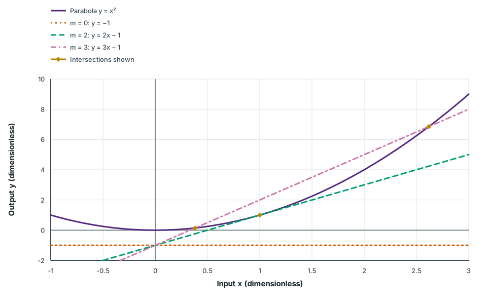
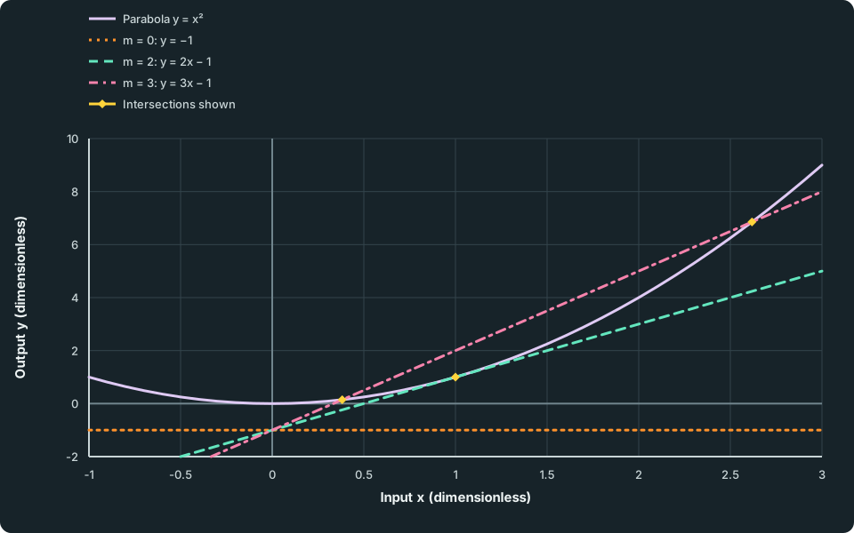
For the line y = mx-1 and curve y = x², substitution gives x² − mx + 1 = 0, with D = m² − 4. Thus there are two distinct real intersections for m < −2 or m > 2, one tangent intersection for m = −2 or 2, and none for −2 < m < 2.
Scroll across the figure to read all labels.
View figure data
| Series | Input x (dimensionless) | Output y (dimensionless) |
|---|---|---|
| Parabola y = x² | -1.00000 | 1.00000 |
| Parabola y = x² | -0.90000 | 0.81000 |
| Parabola y = x² | -0.80000 | 0.64000 |
| Parabola y = x² | -0.70000 | 0.49000 |
| Parabola y = x² | -0.60000 | 0.36000 |
| Parabola y = x² | -0.50000 | 0.25000 |
| Parabola y = x² | -0.40000 | 0.16000 |
| Parabola y = x² | -0.30000 | 0.09000 |
| Parabola y = x² | -0.20000 | 0.04000 |
| Parabola y = x² | -0.10000 | 0.01000 |
| Parabola y = x² | 0.00000 | 0.00000 |
| Parabola y = x² | 0.10000 | 0.01000 |
| Parabola y = x² | 0.20000 | 0.04000 |
| Parabola y = x² | 0.30000 | 0.09000 |
| Parabola y = x² | 0.40000 | 0.16000 |
| Parabola y = x² | 0.50000 | 0.25000 |
| Parabola y = x² | 0.60000 | 0.36000 |
| Parabola y = x² | 0.70000 | 0.49000 |
| Parabola y = x² | 0.80000 | 0.64000 |
| Parabola y = x² | 0.90000 | 0.81000 |
| Parabola y = x² | 1.00000 | 1.00000 |
| Parabola y = x² | 1.10000 | 1.21000 |
| Parabola y = x² | 1.20000 | 1.44000 |
| Parabola y = x² | 1.30000 | 1.69000 |
| Parabola y = x² | 1.40000 | 1.96000 |
| Parabola y = x² | 1.50000 | 2.25000 |
| Parabola y = x² | 1.60000 | 2.56000 |
| Parabola y = x² | 1.70000 | 2.89000 |
| Parabola y = x² | 1.80000 | 3.24000 |
| Parabola y = x² | 1.90000 | 3.61000 |
| Parabola y = x² | 2.00000 | 4.00000 |
| Parabola y = x² | 2.10000 | 4.41000 |
| Parabola y = x² | 2.20000 | 4.84000 |
| Parabola y = x² | 2.30000 | 5.29000 |
| Parabola y = x² | 2.40000 | 5.76000 |
| Parabola y = x² | 2.50000 | 6.25000 |
| Parabola y = x² | 2.60000 | 6.76000 |
| Parabola y = x² | 2.70000 | 7.29000 |
| Parabola y = x² | 2.80000 | 7.84000 |
| Parabola y = x² | 2.90000 | 8.41000 |
| Parabola y = x² | 3.00000 | 9.00000 |
| m = 0: y = −1 | -1.00000 | -1.00000 |
| m = 0: y = −1 | 3.00000 | -1.00000 |
| m = 2: y = 2x − 1 | -0.50000 | -2.00000 |
| m = 2: y = 2x − 1 | -0.40000 | -1.80000 |
| m = 2: y = 2x − 1 | -0.30000 | -1.60000 |
| m = 2: y = 2x − 1 | -0.20000 | -1.40000 |
| m = 2: y = 2x − 1 | -0.10000 | -1.20000 |
| m = 2: y = 2x − 1 | 0.00000 | -1.00000 |
| m = 2: y = 2x − 1 | 0.10000 | -0.80000 |
| m = 2: y = 2x − 1 | 0.20000 | -0.60000 |
| m = 2: y = 2x − 1 | 0.30000 | -0.40000 |
| m = 2: y = 2x − 1 | 0.40000 | -0.20000 |
| m = 2: y = 2x − 1 | 0.50000 | 0.00000 |
| m = 2: y = 2x − 1 | 0.60000 | 0.20000 |
| m = 2: y = 2x − 1 | 0.70000 | 0.40000 |
| m = 2: y = 2x − 1 | 0.80000 | 0.60000 |
| m = 2: y = 2x − 1 | 0.90000 | 0.80000 |
| m = 2: y = 2x − 1 | 1.00000 | 1.00000 |
| m = 2: y = 2x − 1 | 1.10000 | 1.20000 |
| m = 2: y = 2x − 1 | 1.20000 | 1.40000 |
| m = 2: y = 2x − 1 | 1.30000 | 1.60000 |
| m = 2: y = 2x − 1 | 1.40000 | 1.80000 |
| m = 2: y = 2x − 1 | 1.50000 | 2.00000 |
| m = 2: y = 2x − 1 | 1.60000 | 2.20000 |
| m = 2: y = 2x − 1 | 1.70000 | 2.40000 |
| m = 2: y = 2x − 1 | 1.80000 | 2.60000 |
| m = 2: y = 2x − 1 | 1.90000 | 2.80000 |
| m = 2: y = 2x − 1 | 2.00000 | 3.00000 |
| m = 2: y = 2x − 1 | 2.10000 | 3.20000 |
| m = 2: y = 2x − 1 | 2.20000 | 3.40000 |
| m = 2: y = 2x − 1 | 2.30000 | 3.60000 |
| m = 2: y = 2x − 1 | 2.40000 | 3.80000 |
| m = 2: y = 2x − 1 | 2.50000 | 4.00000 |
| m = 2: y = 2x − 1 | 2.60000 | 4.20000 |
| m = 2: y = 2x − 1 | 2.70000 | 4.40000 |
| m = 2: y = 2x − 1 | 2.80000 | 4.60000 |
| m = 2: y = 2x − 1 | 2.90000 | 4.80000 |
| m = 2: y = 2x − 1 | 3.00000 | 5.00000 |
| m = 3: y = 3x − 1 | -0.33333 | -2.00000 |
| m = 3: y = 3x − 1 | -0.25000 | -1.75000 |
| m = 3: y = 3x − 1 | -0.16667 | -1.50000 |
| m = 3: y = 3x − 1 | -0.08333 | -1.25000 |
| m = 3: y = 3x − 1 | 0.00000 | -1.00000 |
| m = 3: y = 3x − 1 | 0.08333 | -0.75000 |
| m = 3: y = 3x − 1 | 0.16667 | -0.50000 |
| m = 3: y = 3x − 1 | 0.25000 | -0.25000 |
| m = 3: y = 3x − 1 | 0.33333 | 0.00000 |
| m = 3: y = 3x − 1 | 0.41667 | 0.25000 |
| m = 3: y = 3x − 1 | 0.50000 | 0.50000 |
| m = 3: y = 3x − 1 | 0.58333 | 0.75000 |
| m = 3: y = 3x − 1 | 0.66667 | 1.00000 |
| m = 3: y = 3x − 1 | 0.75000 | 1.25000 |
| m = 3: y = 3x − 1 | 0.83333 | 1.50000 |
| m = 3: y = 3x − 1 | 0.91667 | 1.75000 |
| m = 3: y = 3x − 1 | 1.00000 | 2.00000 |
| m = 3: y = 3x − 1 | 1.08333 | 2.25000 |
| m = 3: y = 3x − 1 | 1.16667 | 2.50000 |
| m = 3: y = 3x − 1 | 1.25000 | 2.75000 |
| m = 3: y = 3x − 1 | 1.33333 | 3.00000 |
| m = 3: y = 3x − 1 | 1.41667 | 3.25000 |
| m = 3: y = 3x − 1 | 1.50000 | 3.50000 |
| m = 3: y = 3x − 1 | 1.58333 | 3.75000 |
| m = 3: y = 3x − 1 | 1.66667 | 4.00000 |
| m = 3: y = 3x − 1 | 1.75000 | 4.25000 |
| m = 3: y = 3x − 1 | 1.83333 | 4.50000 |
| m = 3: y = 3x − 1 | 1.91667 | 4.75000 |
| m = 3: y = 3x − 1 | 2.00000 | 5.00000 |
| m = 3: y = 3x − 1 | 2.08333 | 5.25000 |
| m = 3: y = 3x − 1 | 2.16667 | 5.50000 |
| m = 3: y = 3x − 1 | 2.25000 | 5.75000 |
| m = 3: y = 3x − 1 | 2.33333 | 6.00000 |
| m = 3: y = 3x − 1 | 2.41667 | 6.25000 |
| m = 3: y = 3x − 1 | 2.50000 | 6.50000 |
| m = 3: y = 3x − 1 | 2.58333 | 6.75000 |
| m = 3: y = 3x − 1 | 2.66667 | 7.00000 |
| m = 3: y = 3x − 1 | 2.75000 | 7.25000 |
| m = 3: y = 3x − 1 | 2.83333 | 7.50000 |
| m = 3: y = 3x − 1 | 2.91667 | 7.75000 |
| m = 3: y = 3x − 1 | 3.00000 | 8.00000 |
| Intersections shown | 1.00000 | 1.00000 |
| Intersections shown | 0.38197 | 0.14590 |
| Intersections shown | 2.61803 | 6.85410 |
At m = 2, the equation is (x − 1)² = 0, giving the tangent point (1,1). At m = −2 it is (x + 1)² = 0, giving (−1,1). At m = 0 the line y = −1 stays below y = x², so no real intersection is possible. These checks connect the algebraic boundary to the original graphs.
The tangent criterion here relies on the genuine quadratic obtained after substitution. For a more general curve, or a parameter value that makes it a line, one real intersection alone need not establish tangency. First identify the actual equation left to solve.
Roots divide the sign intervals
An inequality asks for every input giving the required sign, not just the inputs where the expression is zero. Solve x² + x − 2 ≤ 0 by factoring to (x + 2)(x − 1) ≤ 0. Its roots −2 and 1 separate intervals where the signs of the factors stay fixed:
| Interval | Sign of x + 2 | Sign of x − 1 | Product |
|---|---|---|---|
| x < −2 | Negative | Negative | Positive |
| −2 < x < 1 | Positive | Negative | Negative |
| x > 1 | Positive | Positive | Positive |
The required solution is −2 ≤ x ≤ 1. Include both roots because equality is allowed. On a number line, mark filled circles at −2 and 1 and shade the segment between them. For a strict inequality, use open circles instead: the endpoints would not satisfy it.
The leading sign matters. For −(x + 2)(x − 1) > 0, multiplication by −1 reverses the product’s signs, so the solution is −2 < x < 1. It would be wrong to keep an “outside the roots” rule just because the displayed expression is quadratic.
A repeated root does not reverse the sign
For (x − 1)², both factors change sign together at x = 1. Their product remains positive on either side and is zero at that input. Thus (x − 1)² ≤ 0 has only the solution x = 1, while (x − 1)² < 0 has no solution. On a number line the first is one filled point, rather than a shaded interval. The inequality (x − 1)² > 0 includes every real input except 1, represented by two rays with an open circle at 1.
An inequality’s direction, strictness, leading coefficient and repeated roots all matter. A sketch or factor-sign check decides which intervals to include; the roots alone do not.
Check your understanding 1 Do not discard the outside intervals
Solve 2x²-5x-3 > 0 and represent your solution on a number line. Explain which endpoints are excluded and why the answer needs “or” rather than “and”.
Show answer
Factor to (2x + 1)(x-3) > 0. The roots are −1/2 and 3. A positive product occurs outside them: x < -1/2 or x > 3. The strict inequality excludes both roots. Use open circles at −1/2 and 3, shade left of the first and right of the second, and use outward arrows to show the unbounded rays.
“Or” joins the two separate permitted sets. Requiring x < −1/2 and x > 3 would permit no real input, which does not describe this product’s positive regions.
A parameter may change the degree
For p x² + 2x + 1 = 0, the displayed discriminant is 4 − 4p. At p = 0 this is positive, but the equation has become 2x + 1 = 0, with just one solution x = −1/2. Applying a two-root conclusion there would have used a quadratic theorem after the quadratic term disappeared.
Separate any parameter value that makes the leading coefficient zero, solve that reduced equation directly, and use the discriminant only for the remaining genuine quadratics. A constant equation could have no solutions or every real input; inspect what actually remains rather than assuming it is always linear.
Try it yourself 1
Check what the parameter changes
Problem
The parameter k is real. Find every value of k for which (k-1)x² + 2x + 1 = 0 has exactly one real solution in x. For each such value of k, solve (k-1)x² + 2x + 1 ≤ 0 and represent the solution on a number line.
Explain why the equation’s one-root answer does not by itself determine the entire inequality solution.
Write your answer, then compare it with the solution
Hints
Hint 1
Identify the equation before counting its roots
Check whether any parameter value changes the degree. For the remaining values, decide what discriminant condition gives the requested root count. Return to each original expression when solving the inequality.
Show full solution
Separate the reduced equation
Method
Check k = 1 before applying a quadratic test.Reason
It makes the x² coefficient zero, so it is outside the discriminant theorem’s assumption.Working
Answer
At k = 1 the equation is 2x + 1 = 0, with exactly one real solution x = −1/2. This parameter value must be kept.Find the genuine quadratic with a repeated root
Method
For k ≠ 1, set its discriminant equal to zero.Reason
A genuine quadratic has one distinct real solution exactly in the repeated-root case.Working
Answer
D = 2²-4(k-1) = 4(2-k), so D = 0 gives k = 2. The equation then becomes (x + 1)² = 0, with root x = −1. Thus the complete parameter set is k = 1 or k = 2. Other genuine quadratics have two distinct real roots or none.Solve each inequality using its actual expression
Method
Substitute each permitted k into the original inequality.Reason
A linear crossing and a touching quadratic have different sign regions despite each having one equation solution.Working
Answer
At k = 1, 2x + 1 ≤ 0 gives x ≤ −1/2: a filled circle at −1/2 with the ray to its left shaded. At k = 2, (x + 1)² ≤ 0 holds only at x = −1: a single filled point. The first inequality has infinitely many inputs even though its equation has only one root.
Quick check
Check the degree, parameter condition and each inequality separately. A root locates equality; the sign of the actual expression decides what else belongs to the solution.
Keep track of this lesson
Mark the lesson done when you have worked through it.
Lesson progress is optional and kept on this device.
Loading lesson controls…
Your lesson mark records your own study. Checks are kept separately in My Learning.