Stationary points, tangents and normals
Interpret derivative signs, classify stationary points, and distinguish local behaviour from extrema on a stated domain.
More
Offline pages
Saved on this device only. Connect at least once every 30 days to confirm Premium. Sign-out or a change of account removes saved copies.
Find this activity in your course
On this page
You stopped at:
ContinueRevision Mode is on. Questions and activities are hidden.
A zero derivative gives a point to investigate
The height f(a) locates a point on a curve; the derivative f'(a) gives its tangent gradient. Where f' > 0, the function increases as x increases; where f' < 0, it decreases. A stationary point has f'(a) = 0, but its full coordinates are (a,f(a)). Zero gradient does not mean zero height, and it does not by itself establish a maximum or minimum.
For f(x) = x³-3x,
The stationary inputs are -1 and 1. Substituting into f gives points (-1,2) and (1,-2). The derivative signs are:
| Interval | Sign of f' | Behaviour of f |
|---|---|---|
| x < -1 | Positive | Increasing |
| -1 < x < 1 | Negative | Decreasing |
| x > 1 | Positive | Increasing |
At x = -1, f changes from increasing to decreasing, so (-1,2) is a local maximum. At x = 1, it changes from decreasing to increasing, so (1,-2) is a local minimum. The sign change is the reason for each classification, not merely the equation f' = 0.
The second derivative describes how the gradient changes
The derivative graph’s height represents the original graph’s slope. Differentiating that slope gives f''. A positive second derivative means the tangent gradients increase as x increases: the graph is concave upward. A negative second derivative means those gradients decrease: the graph is concave downward.
This is a different question from whether f itself rises or falls. For f(x) = x², f'(x) = 2x and f''(x) = 2. On the negative half-line, f decreases even though its gradients are increasing from more negative to less negative values. It is concave upward on both sides of the origin.
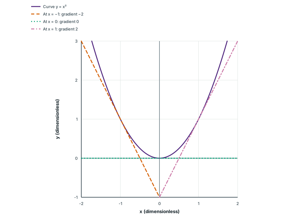
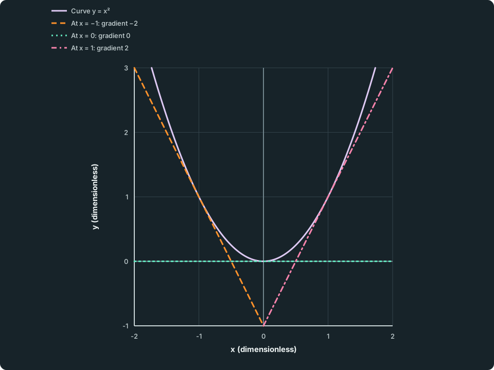
Increasing tangent gradients on y = x²
The upward-opening parabola has a dashed tangent y = −2x − 1 at (−1, 1), a dotted horizontal tangent y = 0 at (0, 0), and a dash-dot tangent y = 2x − 1 at (1, 1). Equal coordinate scales preserve their directions.
Scroll across the figure to read all labels.
View figure data
| Series | x (dimensionless) | y (dimensionless) |
|---|---|---|
| Curve y = x² | -1.73205 | 3.0000000 |
| Curve y = x² | -1.71875 | 2.9541016 |
| Curve y = x² | -1.68750 | 2.8476563 |
| Curve y = x² | -1.65625 | 2.7431641 |
| Curve y = x² | -1.62500 | 2.6406250 |
| Curve y = x² | -1.59375 | 2.5400391 |
| Curve y = x² | -1.56250 | 2.4414063 |
| Curve y = x² | -1.53125 | 2.3447266 |
| Curve y = x² | -1.50000 | 2.2500000 |
| Curve y = x² | -1.46875 | 2.1572266 |
| Curve y = x² | -1.43750 | 2.0664063 |
| Curve y = x² | -1.40625 | 1.9775391 |
| Curve y = x² | -1.37500 | 1.8906250 |
| Curve y = x² | -1.34375 | 1.8056641 |
| Curve y = x² | -1.31250 | 1.7226563 |
| Curve y = x² | -1.28125 | 1.6416016 |
| Curve y = x² | -1.25000 | 1.5625000 |
| Curve y = x² | -1.21875 | 1.4853516 |
| Curve y = x² | -1.18750 | 1.4101563 |
| Curve y = x² | -1.15625 | 1.3369141 |
| Curve y = x² | -1.12500 | 1.2656250 |
| Curve y = x² | -1.09375 | 1.1962891 |
| Curve y = x² | -1.06250 | 1.1289063 |
| Curve y = x² | -1.03125 | 1.0634766 |
| Curve y = x² | -1.00000 | 1.0000000 |
| Curve y = x² | -0.96875 | 0.9384766 |
| Curve y = x² | -0.93750 | 0.8789063 |
| Curve y = x² | -0.90625 | 0.8212891 |
| Curve y = x² | -0.87500 | 0.7656250 |
| Curve y = x² | -0.84375 | 0.7119141 |
| Curve y = x² | -0.81250 | 0.6601563 |
| Curve y = x² | -0.78125 | 0.6103516 |
| Curve y = x² | -0.75000 | 0.5625000 |
| Curve y = x² | -0.71875 | 0.5166016 |
| Curve y = x² | -0.68750 | 0.4726563 |
| Curve y = x² | -0.65625 | 0.4306641 |
| Curve y = x² | -0.62500 | 0.3906250 |
| Curve y = x² | -0.59375 | 0.3525391 |
| Curve y = x² | -0.56250 | 0.3164063 |
| Curve y = x² | -0.53125 | 0.2822266 |
| Curve y = x² | -0.50000 | 0.2500000 |
| Curve y = x² | -0.46875 | 0.2197266 |
| Curve y = x² | -0.43750 | 0.1914063 |
| Curve y = x² | -0.40625 | 0.1650391 |
| Curve y = x² | -0.37500 | 0.1406250 |
| Curve y = x² | -0.34375 | 0.1181641 |
| Curve y = x² | -0.31250 | 0.0976563 |
| Curve y = x² | -0.28125 | 0.0791016 |
| Curve y = x² | -0.25000 | 0.0625000 |
| Curve y = x² | -0.21875 | 0.0478516 |
| Curve y = x² | -0.18750 | 0.0351563 |
| Curve y = x² | -0.15625 | 0.0244141 |
| Curve y = x² | -0.12500 | 0.0156250 |
| Curve y = x² | -0.09375 | 0.0087891 |
| Curve y = x² | -0.06250 | 0.0039063 |
| Curve y = x² | -0.03125 | 0.0009766 |
| Curve y = x² | 0.00000 | 0.0000000 |
| Curve y = x² | 0.03125 | 0.0009766 |
| Curve y = x² | 0.06250 | 0.0039063 |
| Curve y = x² | 0.09375 | 0.0087891 |
| Curve y = x² | 0.12500 | 0.0156250 |
| Curve y = x² | 0.15625 | 0.0244141 |
| Curve y = x² | 0.18750 | 0.0351563 |
| Curve y = x² | 0.21875 | 0.0478516 |
| Curve y = x² | 0.25000 | 0.0625000 |
| Curve y = x² | 0.28125 | 0.0791016 |
| Curve y = x² | 0.31250 | 0.0976563 |
| Curve y = x² | 0.34375 | 0.1181641 |
| Curve y = x² | 0.37500 | 0.1406250 |
| Curve y = x² | 0.40625 | 0.1650391 |
| Curve y = x² | 0.43750 | 0.1914063 |
| Curve y = x² | 0.46875 | 0.2197266 |
| Curve y = x² | 0.50000 | 0.2500000 |
| Curve y = x² | 0.53125 | 0.2822266 |
| Curve y = x² | 0.56250 | 0.3164063 |
| Curve y = x² | 0.59375 | 0.3525391 |
| Curve y = x² | 0.62500 | 0.3906250 |
| Curve y = x² | 0.65625 | 0.4306641 |
| Curve y = x² | 0.68750 | 0.4726563 |
| Curve y = x² | 0.71875 | 0.5166016 |
| Curve y = x² | 0.75000 | 0.5625000 |
| Curve y = x² | 0.78125 | 0.6103516 |
| Curve y = x² | 0.81250 | 0.6601563 |
| Curve y = x² | 0.84375 | 0.7119141 |
| Curve y = x² | 0.87500 | 0.7656250 |
| Curve y = x² | 0.90625 | 0.8212891 |
| Curve y = x² | 0.93750 | 0.8789063 |
| Curve y = x² | 0.96875 | 0.9384766 |
| Curve y = x² | 1.00000 | 1.0000000 |
| Curve y = x² | 1.03125 | 1.0634766 |
| Curve y = x² | 1.06250 | 1.1289063 |
| Curve y = x² | 1.09375 | 1.1962891 |
| Curve y = x² | 1.12500 | 1.2656250 |
| Curve y = x² | 1.15625 | 1.3369141 |
| Curve y = x² | 1.18750 | 1.4101563 |
| Curve y = x² | 1.21875 | 1.4853516 |
| Curve y = x² | 1.25000 | 1.5625000 |
| Curve y = x² | 1.28125 | 1.6416016 |
| Curve y = x² | 1.31250 | 1.7226563 |
| Curve y = x² | 1.34375 | 1.8056641 |
| Curve y = x² | 1.37500 | 1.8906250 |
| Curve y = x² | 1.40625 | 1.9775391 |
| Curve y = x² | 1.43750 | 2.0664063 |
| Curve y = x² | 1.46875 | 2.1572266 |
| Curve y = x² | 1.50000 | 2.2500000 |
| Curve y = x² | 1.53125 | 2.3447266 |
| Curve y = x² | 1.56250 | 2.4414063 |
| Curve y = x² | 1.59375 | 2.5400391 |
| Curve y = x² | 1.62500 | 2.6406250 |
| Curve y = x² | 1.65625 | 2.7431641 |
| Curve y = x² | 1.68750 | 2.8476563 |
| Curve y = x² | 1.71875 | 2.9541016 |
| Curve y = x² | 1.73205 | 3.0000000 |
| At x = −1: gradient −2 | -2.00000 | 3.0000000 |
| At x = −1: gradient −2 | 0.00000 | -1.0000000 |
| At x = 0: gradient 0 | -2.00000 | 0.0000000 |
| At x = 0: gradient 0 | 2.00000 | 0.0000000 |
| At x = 1: gradient 2 | 0.00000 | -1.0000000 |
| At x = 1: gradient 2 | 2.00000 | 3.0000000 |
The tangents at x = -1, 0 and 1 have gradients -2, 0 and 2. Their ordered gradients show what the positive second derivative means. It does not mean that every tangent has a positive gradient or that every function value is increasing.
Check your understanding 1 Direction and curvature answer different questions
For f(x) = x² at x = -1, give f(-1), f'(-1) and f''(-1). Is the function rising or falling there? Are its tangent gradients becoming more negative or less negative as x increases nearby?
Show answer
f(-1) = 1, f'(-1) = -2 and f''(-1) = 2. The function is falling locally because its first derivative is negative. Its gradients become less negative as x increases towards zero, because the second derivative is positive. Positive height, negative slope and upward concavity can occur at the same point.
Use a conclusive test, then explain its limit
At an interior stationary point where the second derivative exists:
| Second derivative at the stationary input | Conclusion |
|---|---|
| f''(a) < 0 | A local maximum |
| f''(a) > 0 | A local minimum |
| f''(a) = 0 | This test is inconclusive |
The stationary condition matters. A positive f''(a) at a point with f'(a) ≠ 0 does not make that point a minimum; it only describes changing slope there.
For f(x) = x³-3x, f''(x) = 6x. At x = -1, the second derivative is negative, confirming the local maximum; at x = 1, it is positive, confirming the local minimum. This agrees with the first-derivative sign test.
For g(x) = x³, however, g'(0) = g''(0) = 0. The first derivative 3x² is positive on both sides of zero, so there is no turn from increasing to decreasing or vice versa. The second derivative 6x changes from negative to positive, giving a stationary point of inflexion at (0,0). The graph changes concavity there while its tangent is horizontal.
Check your understanding 2 A zero second derivative is not a verdict
Classify the stationary point at x = 0 for f(x) = x⁴, then compare g(x) = -x⁴. Explain why knowing only that the first two derivatives vanish at zero does not settle either classification.
Show answer
For f(x) = x⁴, f'(x) = 4x³ changes from negative to positive at zero, so (0,0) is a local minimum. Its nonnegative fourth power also confirms that minimum directly.
For g(x) = -x⁴, g'(x) = -4x³ changes from positive to negative, so (0,0) is a local maximum. Both second derivatives are zero at the stationary input, so the second-derivative test is inconclusive in both cases. Together with the cubic example, these show that zero first and second derivatives can accompany a minimum, a maximum or a stationary point of inflexion.
A tangent needs its point as well as its gradient
A finite tangent gradient m at (a,f(a)) gives
For y = square root of x at x = 4, the point is (4,2) and the derivative is 1/(2 square root of 4) = 1/4. Its tangent is y-2 = (x-4)/4. The normal is perpendicular to that tangent: for finite nonzero m, its gradient is -1/m, giving y-2 = -4(x-4).
At a horizontal tangent, m is zero. The normal is then a vertical line x = a; do not try to assign it the undefined number -1/0 as a gradient. A tangent with zero gradient is still at height f(a), which need not be zero.
Check your understanding 3 Zero gradient does not locate the line’s height
For y = (x-2)² + 5, find the tangent and normal at x = 2. Explain why neither “the tangent is zero” nor a negative-reciprocal calculation alone gives both equations.
Show answer
The point is (2,5) and dy/dx = 2(x-2) = 0 there. The horizontal tangent is y = 5, not y = 0. Its perpendicular normal is x = 2. The point fixes the line positions, and a vertical line has no finite gradient to obtain by dividing by zero.
Check that the point belongs to the original function before using a derivative formula. A cancelled factor can leave an excluded input with no curve point, so extending a simplified derivative there cannot supply a tangent to the original function.
A local extremum need not be the largest or smallest allowed value
A local maximum compares nearby points of the original domain. A global maximum compares every allowed point. On a closed interval for a continuous function, compare all relevant stationary values and endpoint values; also inspect any allowed point where the derivative is undefined. Do not assume every extremum must satisfy f' = 0.
For f(x) = x³-3x restricted to [-3/2,2], the candidates are:
| Input | Reason to check | Function value |
|---|---|---|
| -3/2 | Left endpoint | 9/8 |
| -1 | Stationary input | 2 |
| 1 | Stationary input | -2 |
| 2 | Right endpoint | 2 |
The greatest value is 2, attained at both x = -1 and x = 2. The least is -2 at x = 1. The derivative signs already show the behaviour between candidates, so no larger or smaller interior value is missed. If asked for all points attaining the maximum, giving only the interior local maximum would be incomplete.
Endpoint inclusion also matters. The function f(x) = x on 0 < x < 1 has no greatest value: it approaches the upper bound 1 without attaining it. Reporting the excluded endpoint as an attained maximum changes the domain.
Try it yourself 1
Interpret the supplied derivative
Problem
A differentiable function on the real line has f'(x) = (x-1)²(x + 2), with f(-2) = 1 and f(1) = 31/4. Find and classify its stationary points, and give their tangent and normal equations. Then find the greatest value on the restricted interval [-2,1]. Explain whether the point at the right endpoint is also a local maximum of the original curve.
Write your answer, then compare it with the solution
Hints
Hint 1
Separate a derivative zero from a change of direction
Read the signs on each side of every zero, including the repeated factor. Use the supplied function values to locate the lines, and keep the interval question separate from the whole-curve classification.
Show full solution
Classify the stationary points
Method
Set the supplied derivative equal to zero and inspect its signs.Reason
A repeated zero can leave the derivative’s sign unchanged.Working
Answer
The stationary inputs are -2 and 1. The derivative is negative for x < -2 and positive for -2 < x < 1 and x > 1. Thus (-2,1) is a local minimum. At x = 1 there is no turn; expanding gives f''(x) = 3x²-3, which changes from negative to positive there. Hence (1,31/4) is a stationary point of inflexion.Locate the tangents and normals
Method
Use zero tangent gradient at the two given heights.Reason
Stationarity determines a horizontal direction; the function values determine the tangent positions.Working
Answer
At (-2,1), the tangent is y = 1 and the normal is x = -2. At (1,31/4), the tangent is y = 31/4 and the normal is x = 1.Apply the restricted interval
Method
Use the positive derivative between the two endpoints.Reason
An interval endpoint can be greatest within that interval without being a local maximum of the original curve.Working
Answer
The function increases on (-2,1), so its greatest value on [-2,1] is 31/4 at x = 1. On the original real-line domain it continues increasing past 1, so that stationary point is not a local maximum.
Quick check
The point at x = 1 has three compatible descriptions: a horizontal tangent, a stationary point of inflexion on the original curve, and the greatest value on the selected closed interval. Compare each classification with the domain and the quantity actually requested.
Use the first derivative for direction, the second for changing slope, and a conclusive test for stationary-point classification. Find the curve point before forming a tangent or normal, and compare all allowed candidates when the question asks for a global value.
Keep track of this lesson
Mark the lesson done when you have worked through it.
Lesson progress is optional and kept on this device.
Loading lesson controls…
Your lesson mark records your own study. Checks are kept separately in My Learning.